Understanding RAG and Vector Databases

Or: “How my previous life as an Oracle University Instructor teaching Oracle Spatial, gave me a great start on understanding how RAG interacts with Vector Databases”

I know that is a very long title for an article about GenAI RAG and vector databases. Many years ago, I picked up the Oracle Spatial 3-day course. It took me a little while to get my head around what it was all about, (I did question my life choices a few times) and how Oracle managed to model and use 2 and 3 dimensional spatial data, in tables, made up of rows and columns. But I managed to understand it enough to even explain the magic to others. Let us see if I still have that ability.

In recent years, vector databases have emerged as a powerful tool for working with large-scale, unstructured data, particularly in the field of natural language processing (NLP). This article explains how the Retrieval-Augmented Generation (RAG) models leverage vector databases to enhance their performance. I will be delving into the intricacies of encoding, indexing, query encoding, retrieval, and generation – the steps performed when we use RAG. It examines what unique characteristics of vector databases make them well-suited for this type of work and provides a comprehensive overview of the various steps involved in the RAG process.

What are Vector Databases?

Vector databases are a specialized type of database designed to store and retrieve high-dimensional vector representations of data. Unlike traditional databases that store data in tables with rows and columns, vector databases store data as dense vectors, typically generated by machine learning models. These vectors capture the semantic relationships between data points, allowing for efficient similarity searches and retrieval.

Vector databases are particularly useful in Natural Language Processing (NLP) tasks because they can store and retrieve vector representations of text, such as word embeddings or sentence embeddings. These vector representations capture the semantic meaning of text, enabling more accurate and meaningful comparisons and retrieval than traditional keyword-based searches.

Encoding Techniques

Before data can be stored in a vector database, it must first be encoded into a vector representation. This process typically involves using a pre-trained language model or encoder to generate embeddings for the input text. The embeddings capture the semantic meaning of the text and are represented as high-dimensional vectors.

Text Input

The raw text data is provided as input to the encoding process.

Encoding

Text preprocessing: Before encoding, the text data is usually preprocessed to prepare it for the encoding step. This may involve tasks such as tokenization (splitting the text into words or subwords), lowercasing, removing punctuation, stopword removal, and stemming (a crude heuristic process of removing affixes (prefixes and suffixes) from words to obtain their stem or root form. The words “playing”, “played”, and “plays” would be stemmed to “play”.) or lemmatization (a more sophisticated approach that aims to convert a word to its lemma or base form, taking into account the word’s part of speech and the context in which it appears. The words “better” and “best” would be lemmatized to “good”, and “went” would be lemmatized to “go”.).

Embedding layer: The preprocessed text is then passed through an embedding layer, which converts each word or subword into a dense numerical vector representation. There are several techniques for obtaining these embeddings:

• Pre-trained word embeddings: These are pre-computed word vector representations obtained from models like Word2Vec, GloVe, or FastText, which are trained on large text corpora. These embeddings capture semantic and syntactic relationships between words.
• Contextualized word embeddings: Models like BERT, ELMo, and GPT generate dynamic word embeddings that are sensitive to the context in which the word appears. These models use transformer architectures and self-attention mechanisms to capture context.
• Custom trained embeddings: You can also train your own word embeddings on a domain-specific corpus using techniques like Word2Vec or fastText.

Encoding strategy: After obtaining word-level embeddings, you need to combine them into a single vector representation for the entire text sequence. Common strategies include:

• Mean pooling: Calculate the element-wise mean of all the word embeddings in the sequence.
• Sum pooling: Calculate the element-wise sum of all the word embeddings.
• Max pooling: Take the maximum value along each dimension across all word embeddings.
• Transformer encoder: Pass the word embeddings through a transformer encoder (like in BERT) to obtain a contextualized sequence representation, and then use mean pooling or other strategies on the output.

Indexing Techniques in Vector Databases

Once the data is encoded, it is indexed in the vector database. Indexing involves creating data structures that enable efficient similarity searches and retrieval. Different vector databases may use different indexing techniques, such as k-d trees, hierarchical navigable small world graphs (HNSW), or product quantization. Let me explain each of these in a bit more detail. Other indexing types are used in different Vector DB offerings, but here I will limit myself to just these three.

K-d Trees

The k-d tree data structure is useful for various algorithms that involve multidimensional data, such as nearest neighbour search, range queries, and ray tracing. The performance of operations on a k-d tree depends on the dimensionality of the data and the distribution of the data points.

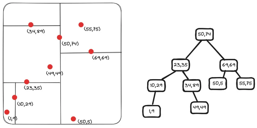
Building a k-d tree (short for k-dimensional tree) is a process of recursively partitioning a k-dimensional space into nested orthogonal half-spaces. The basic idea is to divide the data points into two half-spaces at each level of the tree based on one of the dimensions. A k-d tree can be built like this:

1. Choose the root node: Select the axis (dimension) along which you want to partition the data points. Typically, the axis is chosen in a cyclic or round-robin fashion at each level of the tree.
2. Determine the median: Find the median value of the data points along the chosen axis. This median value will be the splitting value for the current node.
3. Split the data points: Divide the data points into two subsets based on the splitting value. All points with a value less than or equal to the splitting value will go to the left subtree, and all points with a value greater than the splitting value will go to the right subtree.
4. Recursively build subtrees: Recursively apply steps 1-3 on the left and right subsets of data points to build the left and right subtrees, respectively. At each level of the recursion, choose the next axis in a cyclic or round-robin fashion.
5. Termination condition: The recursion stops when a node contains zero or one data point. These nodes are designated as leaf nodes.

Hierarchical Navigable Small World (HNSW) Graphs

HNSW graphs represent a cutting-edge approach to approximate nearest-neighbour search, offering a powerful tool for efficient similarity retrieval in high-dimensional spaces. Their hierarchical and navigable structure makes them particularly well-suited for applications where fast and scalable similarity search is essential, aligning perfectly with the demands of Gen AI technologies.

The idea is that if we take a proximity graph but build it so that we have both long-range and short-range links, then search times are reduced to (poly/)logarithmic complexity.

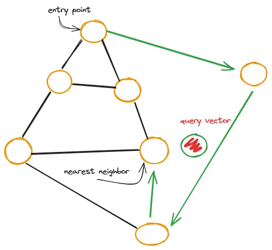
Each vertex in the graph connects to several other vertices. We call these connected vertices friends, and each vertex keeps a friend list, creating our graph.

When searching a Navigable Small World (NSW) graph, we begin at a pre-defined entry-point. This entry point connects to several nearby vertices. We identify which of these vertices is the closest to our query vector and move there.

HNSW is a natural evolution of NSW, which borrows inspiration from hierarchical multi-layers from Pugh’s probability skip list structure. See Appendix A

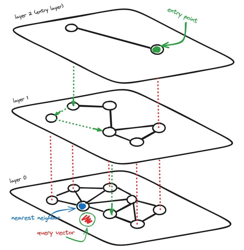
Adding hierarchy to NSW produces a graph where links are separated across different layers. At the top layer, we have the longest links, and at the bottom layer, we have the shortest.

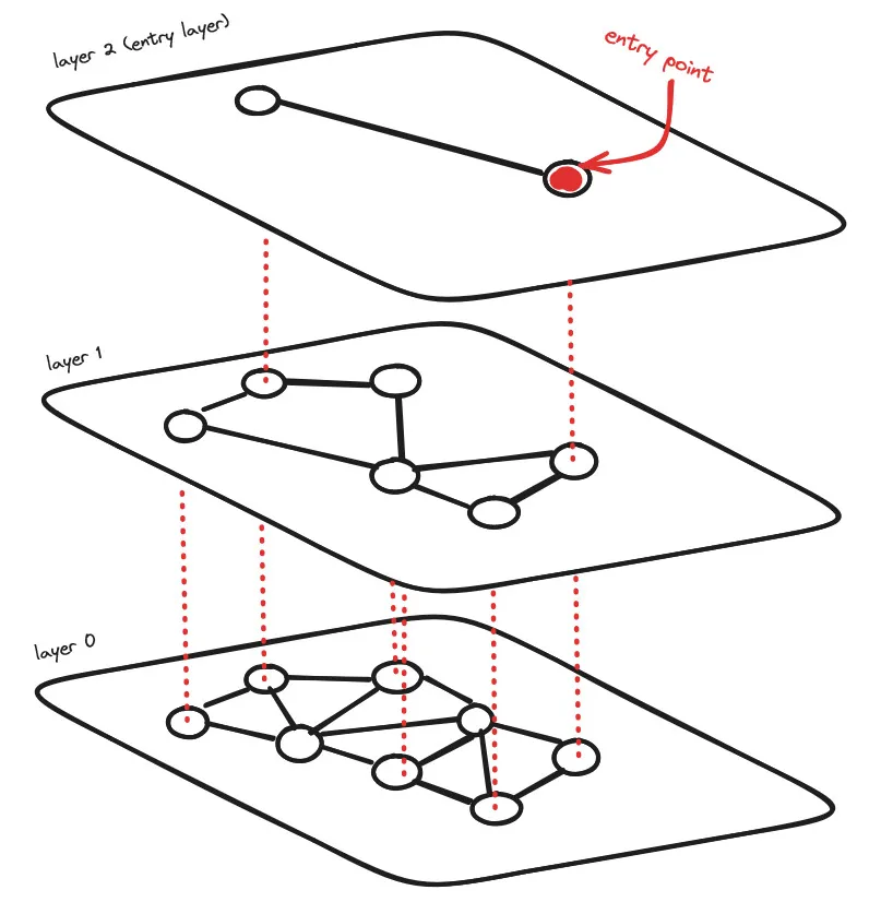
During the search process, we begin at the top layer of the hierarchical navigable small world (HNSW) graph, where we encounter vertices with the longest links. These vertices typically have multiple connections across various layers. This initial phase resembles the zoom-in approach used in the NSW algorithm.

We proceed by traversing edges within each layer, similar to how we did in the NSW algorithm, moving to the nearest vertex at each step until we reach a local minimum. However, unlike in the NSW algorithm, once we reach this local minimum, we transition to the corresponding vertex in a lower layer and continue the search process. We repeat this procedure until we locate the local minimum within our bottom layer, which is typically referred to as layer 0.

Product Quantization (PQ)

PQ is a compression technique that break down vectors into smaller subvectors, allowing for compact storage and fast similarity computations.

Imagine you’re tasked with building a massive knowledge base for a cutting-edge AI system, but the sheer volume of high-dimensional vector data you need to store and process is mind-boggling. You’re facing a classic dilemma: balancing storage efficiency with computational performance. Enter Product Quantization, a compression technique that elegantly tackles this challenge.

At its core, Product Quantization is all about breaking down those high-dimensional vectors into smaller, more manageable subvectors. It’s like taking a large, unwieldy package and breaking it down into smaller, more compact boxes for easier storage and transportation.

Here’s how it works: Let’s say you have a collection of vectors, each with a whopping 512 dimensions. Product Quantization splits each vector into, say, 8 subvectors of 64 dimensions each. Now, instead of storing the original 512-dimensional vector, you can store these 8 subvectors more compactly.

But how, you ask? Well, this is where the quantization part comes in. For each subvector, you have a pre-computed codebook – essentially a lookup table of representative vectors. Each subvector is then encoded as an index into this codebook, representing the closest match.

Imagine you have a codebook with 256 entries for each 64-dimensional subvector. Instead of storing the full 64 float values, you only need to store an 8-bit index pointing to the closest entry in the codebook. That’s a massive compression ratio of 32 times!

Now, you might be thinking, “But won’t this quantization introduce errors and degrade the quality of my precious vector data?” Fair concern, however, Product Quantization is designed to minimize these quantization errors through clever subvector partitioning and codebook learning algorithms.

But the real magic happens during similarity computations. When you need to find the nearest neighbours of a query vector, you can perform efficient distance computations directly on the compressed, quantized representations. No need to decompress the full vectors, saving precious compute cycles and enabling lightning-fast similarity searches.

It’s like having a well-organized warehouse where you can quickly locate the items you need without having to unpack and inspect every single box.

PQ enables compact storage of massive vector collections, facilitating scalability, while also providing fast similarity computations, ensuring snappy performance for your AI applications.

Query Encoding

During inference, when a user submits a query or input text to the RAG model, this text needs to be transformed into a vector representation that can be compared with the vectors in the knowledge base. This transformation process is known as query encoding, and it follows a similar approach to the encoding of the knowledge base texts.

Allow me to walk you through the query encoding process step-by-step:

1. Tokenization: Just like with the knowledge base texts, the user’s input query is first tokenized into a sequence of tokens.
2. Token Embedding: Each token in the query sequence is then mapped to a dense vector representation using the same token embedding model that was used for encoding the knowledge base texts.
3. Contextual Encoding: The sequence of token embeddings for the query is then passed through the same pre-trained language model (e.g., BERT, RoBERTa, GPT) that was used for encoding the knowledge base texts.
4. Pooling or Aggregation: Similar to the knowledge base encoding, the contextualized token representations for the query are pooled or aggregated into a single vector representation. Common pooling methods include mean pooling (taking the mean of all token vectors), max pooling (taking the maximum value along each dimension), or using specialized pooling mechanisms like the [CLS] token in BERT models.

It’s crucial to note that the same encoding model (e.g., BERT, RoBERTa, GPT) and pooling mechanism used for encoding the knowledge base texts must be used for encoding the query. This ensures that the vector representations are in the same semantic space, enabling meaningful similarity comparisons and retrieval of relevant information from the vector database.

The resulting query vector representation captures the semantic meaning of the user’s input query and can be used for similarity search in the vector database to retrieve the most relevant encoded texts from the knowledge base.

By following this query encoding process, the RAG model can effectively translate the user’s input into a high-dimensional vector representation that can be compared with the vectors in the knowledge base, enabling the retrieval of relevant information to inform the model’s generation process.

It’s worth mentioning that while the query encoding process is computationally less expensive than encoding the entire knowledge base, it still requires substantial computational resources, especially when dealing with large language models and high-dimensional vectors. Efficient implementation and optimizations are crucial for ensuring real-time performance in production environments.

Retrieval

In the retrieval phase, the encoded query vector is used to search the vector database for the most relevant pieces of information from the knowledge base.

You should already understand the importance of efficient data retrieval and indexing strategies for large-scale systems. The retrieval process in RAG models leverages specialized indexing techniques and algorithms to enable fast and accurate similarity searches on high-dimensional vector representations.

Here’s a detailed breakdown of the retrieval process:

1. Index Loading: Before performing the similarity search, the relevant index(es) from the vector database needs to be loaded into memory. Recall that during the indexing step, the vector representations of the knowledge base texts were partitioned and indexed using various data structures, such as flat indexes, tree-based indexes (e.g., k-d trees, HNSW graphs), or quantization-based indexes (e.g., Product Quantization, Scalar Quantization).

The specific index(es) to load depends on the partitioning strategy and the characteristics of the query vector. For example, if the knowledge base vectors were partitioned based on semantic similarity, the index(es) corresponding to the most relevant partition(s) for the query would be loaded.

2. Similarity Search: With the relevant index(es) loaded into memory, the encoded query vector is used to traverse the index data structure(s) and perform a similarity search. The goal is to find the nearest neighbour vectors, which correspond to the most similar encoded texts from the knowledge base.

The similarity search algorithms employed by vector databases are optimized for high-dimensional vector spaces and can efficiently prune irrelevant portions of the index, reducing the number of distance computations required.

Common similarity search algorithms include:

• Exact Nearest Neighbour Search: This approach finds the exact nearest neighbours by computing the distance between the query vector and all vectors in the index. While accurate, it can be computationally expensive for large datasets.
• Approximate Nearest Neighbour Search: These algorithms trade off a small amount of accuracy for significant performance gains by approximating the nearest neighbours. Popular examples include Locality-Sensitive Hashing (LSH), Hierarchical Navigable Small World (HNSW) graphs, and Product Quantization.

3. Result Retrieval: After traversing the index data structure(s), the similarity search algorithm returns the top-k nearest neighbour vectors to the query vector. These top-k vectors correspond to the most relevant encoded texts from the knowledge base, based on their semantic similarity to the query.

Each retrieved vector is associated with metadata, such as the original text or document ID, allowing the RAG model to retrieve the actual textual information from the knowledge base.

For example, let’s assume the query “Charlotte went to Paris, to learn French?” is encoded into a vector q. The similarity search on the vector database might return the top-5 nearest neighbour vectors, corresponding to encoded texts like:

1. “Many students choose to study abroad in Paris to immerse themselves in the French language and culture”.
2. “Learning a new language is often easier and more effective when you’re surrounded by native speakers, which is why Paris is a popular destination for those wanting to learn French”.
3. “Immersion programs in Paris offer intensive French language courses combined with cultural activities and opportunities to practice conversation with locals”.
4. “For those serious about mastering French, living and studying in a French-speaking city like Paris is often recommended as it forces you to use the language daily”.
5. “Paris has a wide range of language schools catering to different levels and learning styles, from intensive group classes to private tutoring”.

These relevant encoded texts, along with their associated metadata, are then passed on to the generation step of the RAG model.

It’s important to note that the retrieval process is highly dependent on the quality and coverage of the indexed knowledge base, as well as the effectiveness of the encoding and indexing strategies employed. Techniques like retrieval augmentation, where multiple retrieval strategies are combined, can further improve the quality and diversity of the retrieved information.

Additionally, efficient implementation and optimization of the similarity search algorithms are crucial for achieving real-time performance, especially when dealing with large-scale knowledge bases and high-dimensional vector spaces.

By leveraging specialized indexing techniques and similarity search algorithms, the retrieval step in RAG models enables efficient and accurate retrieval of relevant information from the knowledge base, which is then used to inform and augment the generation process, resulting in more knowledgeable and context-aware outputs.

Generation

We are finally at the culmination of the retrieval-augmented process. It is here the retrieved relevant information and the original query are synthesized to produce the final output text.

You very likely understand the importance of seamlessly integrating various components and leveraging the strengths of different technologies to achieve a cohesive and effective system.

In the context of RAG models, the generation step involves feeding the retrieved relevant information and the original query into a transformer-based language model, which then generates the final output text, potentially incorporating the retrieved knowledge into its response.

Let’s break down this process in more detail:

1. Input Preparation: The first step is to prepare the input for the transformer-based language model. This typically involves concatenating the original query or input text with the relevant information retrieved from the vector database. For example, if the query is “Charlotte went to Paris, to learn French”, and the retrieved information includes texts like “Paris, being a global center of French culture and language” and “By living amongst native French speakers and being constantly exposed to the language in daily life, Charlotte will likely acquire French much faster compared to classroom-only instruction”., these texts would be concatenated with the query to form the input for the language model.
2. Language Model Selection: The choice of the transformer-based language model can vary depending on the specific implementation and requirements of the RAG model. Popular choices include pre-trained models like GPT (Generative Pre-trained Transformer), BART (Bidirectional and Auto-Regressive Transformer), or custom models trained specifically for the task at hand.
3. Generation Process: The prepared input is then fed into the chosen transformer-based language model, which generates the final output text. The generation process typically involves auto-regressive decoding, where the model generates one token (word or subword) at a time, conditioned on the input and the previously generated tokens.
   During this process, the language model can incorporate the retrieved relevant information into its output, synthesizing and presenting the knowledge in a coherent and natural manner. The model’s attention mechanism and ability to capture long-range dependencies enable it to effectively utilize the retrieved information and generate context-aware responses.
4. Output Post-processing: Depending on the specific implementation, the generated output may undergo post-processing steps, such as filtering out inappropriate or offensive content, enforcing length constraints, or applying formatting rules.

For example, let’s assume the input to the language model is “Charlotte went to Paris, to learn French”, “Paris, being a global center of French culture and language” and “By living amongst native French speakers and being constantly exposed to the language in daily life, Charlotte will likely acquire French much faster compared to classroom-only instruction”.. The language model might generate an output like:

“Charlotte made the smart decision to travel to Paris to learn French through full immersion. Paris, being a global center of French culture and language, offers numerous highly-rated language schools that provide intensive immersive programs. By living amongst native French speakers and being constantly exposed to the language in daily life, Charlotte will likely acquire French much faster compared to classroom-only instruction. Immersive language learning has been shown to greatly accelerate vocabulary acquisition, improve listening comprehension, and help learners gain a more natural grasp of pronunciation and conversational nuances.”

In this example, the language model has effectively incorporated the retrieved relevant information about travelling to Paris to learn French is a good idea synthesized additional details and context to provide a comprehensive and informative response.

It’s important to note that the quality and coherence of the generated output heavily depend on the capabilities of the transformer-based language model, the quality and relevance of the retrieved information, and the effectiveness of the input preparation and integration strategies.

Additionally, language models can sometimes exhibit undesirable behaviors, such as hallucinating or generating factually incorrect information, particularly when the retrieved information is incomplete or contradictory. Techniques like constrained decoding, where the model is guided to generate outputs that adhere to certain constraints or facts, can help mitigate these issues.

The generation step in RAG models leverages the power of transformer-based language models to synthesize and present the retrieved relevant information in a natural and coherent manner, enabling the production of knowledge-grounded and context-aware outputs.

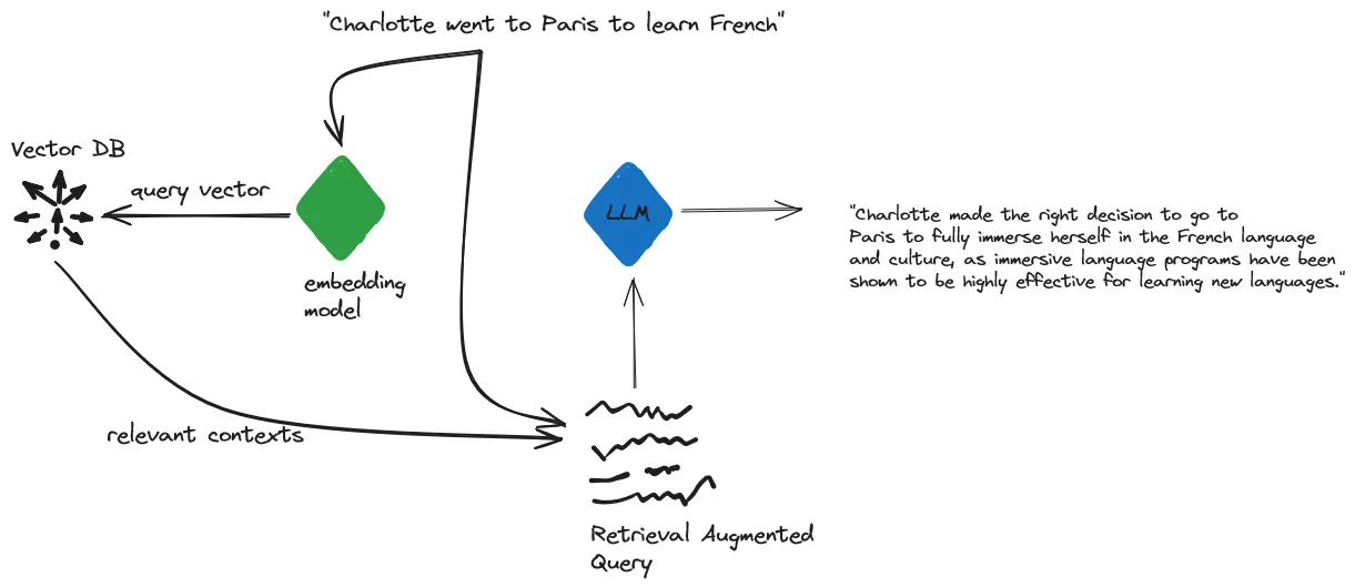
So, if I put the sentence “Charlotte went to Paris to learn French” through RAG, I might get this answer:

“Charlotte made the right decision to go to Paris to fully immerse herself in the French language and culture, as immersive language programs have been shown to be highly effective for learning new languages.”

The key point is that the RAG model can incorporate external knowledge from the retrieved passages while still maintaining coherence with the original input prompt. The generated output vector captures this combined understanding.

The vector representation of the sentence “Charlotte went to Paris, to learn French” would be a dense numerical vector where each element corresponds to a particular feature or dimension of the input sentence.

The exact vector representation would depend on the specific model architecture and the pre-training corpus used, but in general, it would be a high-dimensional vector, typically with a few hundred or a few thousand elements.

For example, if we were using a BERT-based model pre-trained on a large corpus of text, the vector representation of the sentence “Charlotte went to Paris, to learn French” might look something like this (simplified for illustration purposes):

[0.21, -0.05, 0.14, -0.09, 0.03, ..., 0.18, -0.07, 0.11, 0.05, -0.02]

In this example, each number represents the value of a particular dimension or feature in the vector representation. The specific values would be determined by the model’s understanding of the sentence based on its pre-training on a large corpus of text.

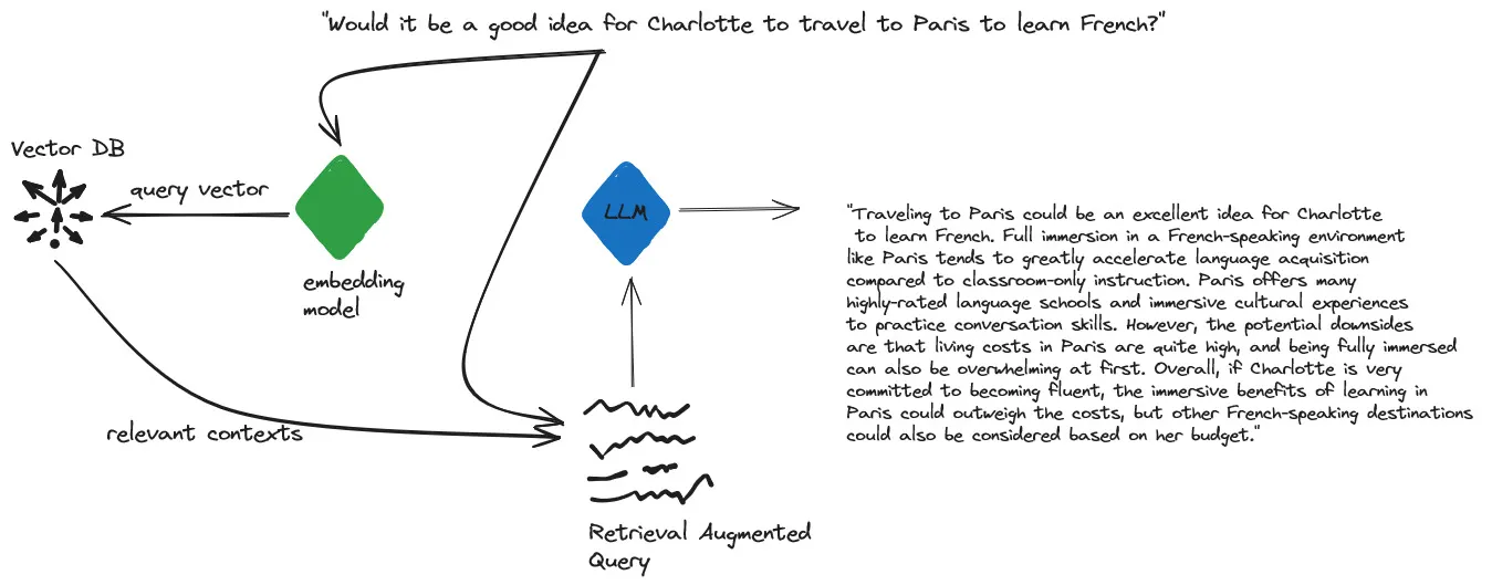
If I change the query slightly: “Would it be a good idea for Charlotte to travel to Paris to learn French?”, the vector representation would be similar in nature to the previous example, but with some differences due to the change in phrasing and context.

Like before, the sentence would be encoded into a high-dimensional dense vector by passing it through a pre-trained transformer-based encoder like BERT or RoBERTa. The specific values in the vector would depend on the model architecture, pre-training corpus, and the contextual understanding of the sentence.

Here’s an example of what the vector representation might look like (again, simplified for illustration purposes):

[0.19, -0.03, 0.12, -0.07, 0.05, ..., 0.16, -0.09, 0.13, 0.07, -0.04]

While the numerical values in this vector would be different from the previous example, there would likely be some similarities in certain dimensions due to the shared context of “Charlotte”, “Paris”, and “learn French”.

However, the presence of the phrase “Would it be a good idea” and the change in sentence structure would likely result in differences in other dimensions of the vector. These differences would capture the nuanced meaning and the interrogative nature of the new sentence, allowing the model to understand and generate appropriate responses based on the encoded representation.

It’s important to note that these vector representations are not easily interpretable by humans, as they exist in a high-dimensional space optimized for machine learning tasks. However, they capture the semantic and contextual information present in the input sentence, allowing the model to perform tasks such as text generation, classification, or retrieval based on the encoded representations.

I hope this explains how RAG uses Vector Databases and a little bit about how the vast amounts of data, all those data points and dimensions are handled. Please let me know if you have any questions or comments.

Appendix

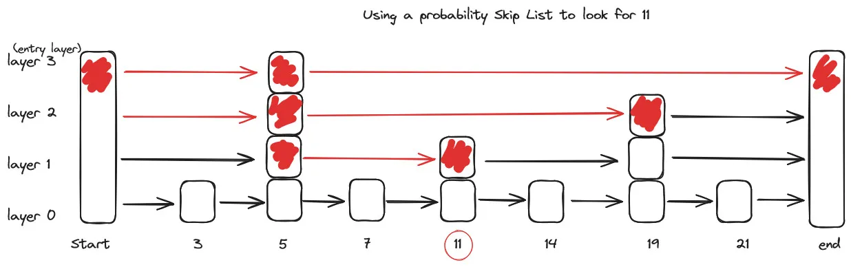
Appendix A: Pugh’s probability skip list structure

Skip lists[1] are data structures that use probabilistic balancing rather than strictly enforced balancing. As a result, the algorithms for insertion and deletion in skip lists are much simpler and significantly faster than equivalent algorithms for balanced trees.

References

[1] “Pugh, W. (1990). Skip lists: a probabilistic alternative to balanced trees. Communications of the ACM, 33(6), pp.668–676.” ‌