Liquid Neural Networks

Chapter 1: Introduction and Background

Liquid Neural Networks represent an exciting evolution in the field of artificial intelligence, combining ideas from traditional neural networks with insights from dynamical systems theory. In this chapter, we introduce the concept and provide the necessary background to understand why liquid models are emerging as powerful tools for handling complex, time-varying data.

What Are Neural Networks?

At their core, neural networks are computational models inspired by the human brain. They consist of layers of interconnected nodes (or neurons) that process information. Traditional neural networks typically operate with fixed architectures, meaning that once a network is trained, its internal parameters remain constant during inference.

The Evolution Toward Liquid Neural Networks

Traditional models have proven effective for many tasks, such as image recognition and language processing. However, they often struggle with dynamic environments where data changes over time or when the system needs to adapt quickly to new information.

Liquid Neural Networks introduce the idea of “liquidity” into the network’s behavior. This concept borrows from fluid dynamics, where the system continuously adapts and evolves. Instead of having fixed weights and static behavior, a liquid network’s internal states can change dynamically over time.

Key Concept: Dynamic Adaptation

Imagine you are trying to predict the weather. The underlying conditions change every minute, and a static model might not be able to keep up with these rapid changes. A liquid neural network, however, is designed to adapt its internal state on the fly. This dynamic adaptation can be thought of as allowing the network to “flow” with the data, similar to how a liquid conforms to the shape of its container.

The Role of Mathematics in Liquid Neural Networks

While the overall ideas are conceptually accessible, there is a strong mathematical backbone behind these networks. In traditional neural networks, you might see formulas such as the following:

This formula represents the output $y$ of a neuron, where $x_i$ are the inputs, $w_i$ are the weights, $b$ is the bias, and $f$ is an activation function.

Liquid Neural Networks extend this idea by incorporating differential equations to model how the network’s state evolves over time. For example, one might encounter an equation like this:

In this equation, $\mathbf{h}(t)$ represents the state of the network at time $t$ , and the equation describes how this state changes continuously over time. The function $\sigma$ serves as an activation function, and $W$ , $U$ , and $\mathbf{b}$ are parameters that help determine the dynamics of the network.

Why “Liquid”?

The term “liquid” is used because these networks can adapt much like a liquid adapts to its container. Their continuously changing internal states enable them to respond in real time to new and evolving data patterns. This makes them particularly well-suited for applications where the data is not static, such as robotics, real-time control systems, and time-series forecasting.

A Glimpse Into the Future

Liquid Neural Networks are still an emerging technology, but their promise lies in their ability to handle real-world complexities that static models may struggle with. As research progresses, we anticipate that these networks will unlock new capabilities and lead to further innovations in AI.

In the following chapters, we will delve deeper into the mathematical foundations, architecture, training strategies, and applications of Liquid Neural Networks. This chapter has provided a high-level overview to set the stage for a deeper exploration of these fascinating models.

Chapter 2: Mathematical and Theoretical Foundations

In this chapter, we explore the core mathematical ideas and theoretical principles that underpin Liquid Neural Networks.

Dynamical Systems and Differential Equations

Liquid Neural Networks are inspired by dynamical systems—systems that change continuously over time. At the heart of this idea is the differential equation. Differential equations describe how a quantity changes with respect to another (often time). A simple example of a differential equation is:

In this formula, $\frac{dy(t)}{dt}$ represents the rate of change of $y(t)$ at time $t$ , and $f(y(t), t)$ is a function that governs this change. This type of equation helps us understand how systems evolve over time.

The Role of Continuous-Time Dynamics

Traditional neural networks typically work in discrete time steps. In contrast, Liquid Neural Networks leverage continuous-time dynamics. This allows them to model systems where changes occur smoothly and continuously. For instance, the evolution of the network’s state can be described by an equation like:

Here:

• $\mathbf{h}(t)$ is the state of the network at time $t$ .
• The term $-\mathbf{h}(t)$ can be seen as a decay or reset mechanism.
• $\sigma$ is an activation function that introduces nonlinearity.
• $W$ and $U$ are weight matrices, while $\mathbf{b}$ is a bias vector.
• $\mathbf{x}(t)$ is the input at time $t$ .

This equation illustrates how the network’s state dynamically evolves, continuously adapting as new data arrives.

Key Mathematical Concepts

To fully grasp Liquid Neural Networks, it helps to be familiar with a few additional mathematical concepts:

• Linear Algebra:
  Understanding vectors and matrices is essential. Operations such as matrix multiplication play a critical role in how inputs are processed within a network.
• Nonlinear Functions:
  Activation functions like the sigmoid or ReLU introduce nonlinearity into the model. These functions ensure that the network can capture complex patterns in the data.
• Stability Analysis:
  In dynamical systems, it is important to know whether a system will settle into a steady state or continue changing unpredictably. Tools from stability analysis help us understand and design networks that behave in a controlled manner.

Bringing It All Together

By combining these mathematical tools, Liquid Neural Networks are able to model environments that evolve continuously over time. Instead of processing data in isolated snapshots, these networks maintain an internal state that flows and adapts, capturing both short-term changes and long-term trends.

The equations and concepts introduced in this chapter form the theoretical backbone for understanding how liquid models operate. As we move to later chapters, we will see how these mathematical principles are applied in practice, guiding the design and training of these adaptive networks.

Chapter 3: Architecture of Liquid Neural Networks

In this chapter, we delve into the architecture that makes Liquid Neural Networks unique. We explain the structure and components of these networks, along with the underlying mechanisms that enable their dynamic behavior.

Overview of Network Components

Liquid Neural Networks build upon the traditional structure of neural networks but introduce elements that allow them to change over time. Their architecture generally includes:

• Neurons: The basic computational units that process incoming signals.
• Connections: Links between neurons through which information flows.
• Dynamic States: Unlike static networks, these have states that evolve continuously.

Dynamic States and Liquid Time-Constants

A defining feature of liquid architectures is their dynamic state. Traditional neural networks use fixed weights once trained, but liquid models incorporate time-dependent dynamics. This means that the state of a neuron, often denoted as $\mathbf{h}(t)$ , is not fixed but evolves according to the network’s ongoing interactions and inputs.

One key component is the concept of liquid time-constants, which enable the network to adjust the rate at which neurons update their state. A simplified dynamic model for a neuron’s state might be expressed as:

In this equation:

• $\mathbf{h}(t)$ is the state of the neuron at time $t$ .
• $\tau$ represents the time constant, controlling the speed of state change.
• The term $-\frac{1}{\tau} \mathbf{h}(t)$ acts as a decay, ensuring that the state does not grow indefinitely.
• $\sigma$ is an activation function that introduces nonlinearity.
• $W$ and $U$ are weight matrices, and $\mathbf{b}$ is the bias.
• $\mathbf{x}(t)$ represents the input at time $t$ .

Layers and Their Interactions

Liquid Neural Networks can be structured in layers, much like conventional networks. However, each layer in a liquid model processes information not only from its immediate inputs but also considers the continuously evolving state of its neurons.

Example of Layered Dynamics

Consider a two-layer liquid neural network where the first layer processes the input data and the second layer refines the output based on the evolving state. The dynamics in the first layer could be described by:

For the second layer, the state evolution might be:

Here:

• $\mathbf{h}^{(1)}(t)$ and $\mathbf{h}^{(2)}(t)$ denote the states of the first and second layers respectively.
• $\tau_1$ and $\tau_2$ are the time constants for the respective layers.
• The equations show how each layer not only reacts to incoming signals but also integrates its own state over time.

Nonlinear Activation and State Evolution

The activation function $\sigma$ is central to enabling complex behaviors within the network. It introduces nonlinearity, which allows the network to capture intricate patterns in the data. Common choices for $\sigma$ include functions like the sigmoid or ReLU. In a liquid network, this activation is applied dynamically, affecting the state evolution continuously.

Architectural Flexibility and Adaptation

One of the strengths of Liquid Neural Networks is their architectural flexibility. By allowing time-dependent adaptation in their internal states, these networks can be tailored to a wide range of tasks that involve temporal data. They can adjust to new patterns on the fly, making them well-suited for applications such as:

• Real-time control systems
• Time-series forecasting
• Robotics and autonomous systems

This flexibility is achieved through a careful balance of the decay mechanisms, dynamic time-constants, and nonlinear activation functions, ensuring that the network can maintain stability while adapting to changing inputs.

In the next chapter, we will explore the training and optimization strategies specific to Liquid Neural Networks, discussing how these dynamic architectures are effectively trained and deployed.

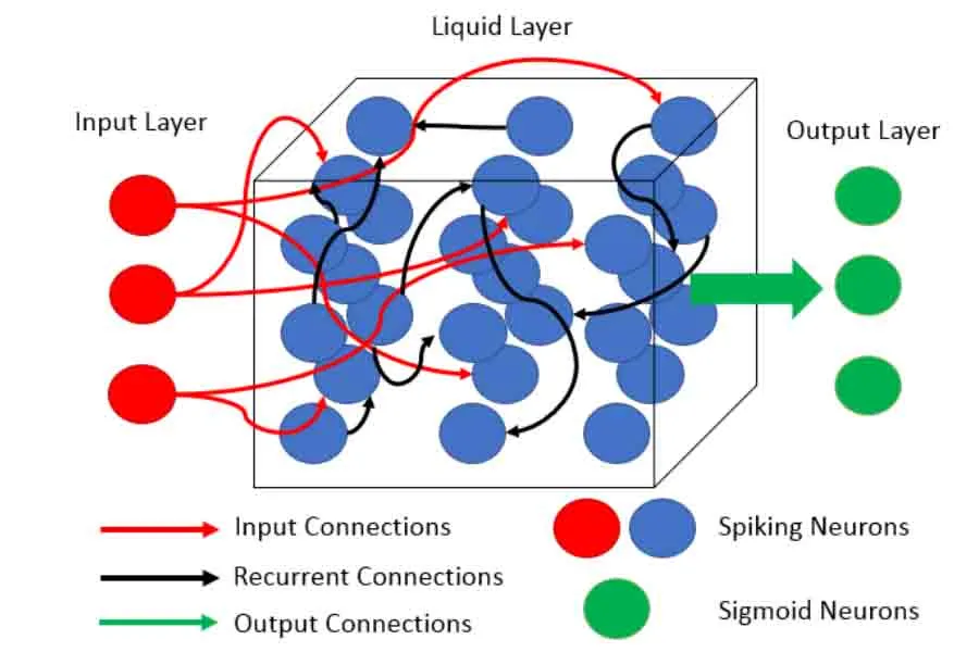
Figure 1. A example of a Liquid Neural Network

Chapter 4: Training and Optimization Strategies

In this chapter, we explore how Liquid Neural Networks are trained and optimized. The goal is to adjust the network’s parameters so that it can adapt its dynamic behavior to perform well on specific tasks, such as time-series prediction or control tasks.

Overview of the Training Process

Training Liquid Neural Networks involves a process similar to that used in traditional neural networks but with additional challenges due to their dynamic nature. The training process typically includes:

• Defining a Loss Function:
  The loss function quantifies how well the network’s predictions match the target outcomes. A common example is the mean squared error (MSE) loss:

  $L = \frac{1}{T} \sum_{t=1}^{T} \left(\hat{y}(t) - y(t)\right)^2$

• Backpropagation Through Time (BPTT):
  Because the network’s state evolves continuously, training requires unfolding the network in time. BPTT is an extension of backpropagation that computes gradients across multiple time steps.

• Gradient-Based Optimization:
  Once gradients are computed, algorithms like stochastic gradient descent (SGD) or Adam are used to update the network’s parameters. The update rule for a parameter $\theta$ might be expressed as:

  $\theta \leftarrow \theta - \eta \frac{\partial L}{\partial \theta}$

  where $\eta$ is the learning rate.

Special Considerations for Liquid Networks

Liquid Neural Networks introduce extra complexities due to their dynamic state evolution:

• Continuous State Adaptation:
  The internal state $\mathbf{h}(t)$ evolves over time according to differential equations. This requires careful handling during training to ensure that the gradient information is propagated accurately over time.
• Stability and Vanishing/Exploding Gradients:
  The continuous nature of the dynamics can lead to issues such as vanishing or exploding gradients. Techniques like gradient clipping or careful initialization of time constants $\tau$ are often necessary.
• Temporal Data Handling:
  Because these networks work with sequences, the training process must manage dependencies across different time steps. This is particularly important in tasks where past information heavily influences future predictions.

Loss Function and Optimization Dynamics

The overall goal is to minimize the loss function $L$ across a sequence of time steps. As the network processes data continuously, the loss function may be integrated over time. An example of a time-integrated loss function is:

This integral form emphasizes that the network’s performance is evaluated continuously rather than at discrete time intervals.

Training Pipeline Overview

The training pipeline for Liquid Neural Networks can be summarized as follows:

1. Data Input:
   Sequences of time-dependent data are fed into the network.
2. Forward Pass:
   The network processes the data through its dynamic state evolution, computing outputs $\hat{y}(t)$ over time.
3. Loss Computation:
   The loss function $L$ is computed by comparing the network outputs to the true values.
4. Backward Pass (BPTT):
   The error is propagated back through time to compute gradients.
5. Parameter Update:
   The network’s parameters (including weights, biases, and time constants) are updated using a gradient-based optimizer.

Figure 2. Training process for Liquid Neural Networks

This graph outlines the step-by-step training process, from data input through forward and backward passes to the parameter update, highlighting how the dynamic nature of the network is handled through BPTT and gradient-based optimization.

In the next chapter, we will explore real-world applications and case studies to see how these training strategies translate into effective performance on challenging tasks.

Chapter 5: Applications and Case Studies

In this chapter, we explore how Liquid Neural Networks are applied across various real-world domains and review case studies that illustrate their unique capabilities.

Applications of Liquid Neural Networks

Liquid Neural Networks excel in scenarios where the data changes continuously over time. Their dynamic state adaptation makes them especially useful in the following areas:

• Time-Series Forecasting:
  Liquid Neural Networks can capture both short-term fluctuations and long-term trends in sequential data. They are ideal for predicting weather patterns, stock market movements, and energy consumption.
• Robotics and Real-Time Control:
  In robotics, rapid adaptation is critical. Liquid Neural Networks are used in control systems where the network must quickly adjust to changing sensor inputs and environmental conditions.
• Autonomous Vehicles:
  Self-driving cars require models that respond immediately to a stream of sensory data. The continuous dynamics of liquid networks help in processing and reacting to real-time information.
• Medical Diagnostics:
  In monitoring patient data over time (e.g., ECG signals), these networks can detect subtle changes and predict critical events.
• Financial Modeling:
  Liquid models can be employed to analyze high-frequency trading data, adapting to market volatility with greater sensitivity than static models.

Case Studies

Time-Series Forecasting

One notable case study involves using Liquid Neural Networks for weather prediction. By continuously updating their internal state based on new sensor data, these networks can improve forecast accuracy over traditional static models.

Example Mathematical Model:

In this model, $\mathbf{h}(t)$ represents the evolving state of the network, capturing the underlying dynamics of weather changes over time.

Robotics and Control Systems

In robotics, Liquid Neural Networks are deployed to manage continuous control tasks. For instance, a robotic arm can use such a network to adjust its movement in response to varying loads or environmental obstacles. The network’s ability to adapt in real time leads to smoother and more precise control.

Autonomous Vehicles

Autonomous vehicles benefit from the dynamic properties of liquid networks. By integrating information from cameras, LiDAR, and other sensors, the network continuously refines its predictions of the vehicle’s surroundings. This results in faster reaction times and improved decision-making in complex traffic scenarios.

Figure 3. Applications of Liquid Neural Networks

This diagram provides an overview of the key domains where liquid networks are making an impact, emphasizing their versatility and dynamic capabilities.

Summary

Liquid Neural Networks are proving to be a powerful tool for tasks that require continuous adaptation and real-time processing. Through various case studies—from weather forecasting to autonomous vehicles—we see how these networks can address challenges that static models struggle with. Their ability to integrate temporal dynamics into predictions makes them especially valuable in complex, time-dependent environments.

Chapter 6: Comparison with Traditional Neural Networks

In this chapter, we compare Liquid Neural Networks with traditional static neural networks. We discuss the benefits and trade-offs of liquid models, focusing on their dynamic behavior versus the fixed structure of conventional networks.

Dynamic vs. Static Architectures

Traditional neural networks have a fixed architecture once training is complete. Their weights remain constant during inference, which can limit their ability to adapt in real time. For instance, a standard neuron in a static network computes its output as:

In contrast, Liquid Neural Networks continuously update their internal state based on new inputs. Their dynamic nature allows them to respond flexibly to time-varying data, as illustrated by the following state evolution equation:

Advantages of Liquid Neural Networks

Adaptability

Liquid networks adjust their state dynamically, making them well-suited for tasks with continuously changing data. This adaptability is especially beneficial for applications like time-series forecasting and real-time control.

Temporal Sensitivity

Because liquid models capture the continuous evolution of their state, they can effectively model long-term dependencies and temporal correlations that static networks might miss.

Improved Robustness

The inherent adaptability of liquid networks can lead to greater robustness in the presence of noisy or rapidly changing inputs. They are better equipped to handle sudden shifts in the data compared to traditional models.

Chapter 7: Performance Comparison Between Liquid Neural Networks and Deep Neural Networks

In this chapter, we examine how Liquid Neural Networks (LNNs) perform in comparison to traditional Deep Neural Networks (DNNs). We explore aspects such as accuracy, adaptability, computational efficiency, and training dynamics.

Accuracy and Adaptability

LNNs have a unique advantage when it comes to handling time-dependent and dynamic data. Their continuously evolving internal states allow them to adapt in real time. This can lead to improved accuracy in tasks such as time-series forecasting and control systems, where traditional DNNs might struggle to capture rapid changes.

For example, the performance of both networks in a forecasting task can be measured using a common metric like Mean Squared Error (MSE). The MSE is defined as:

Here, $y(t)$ represents the true value at time $t$ , and $\hat{y}(t)$ is the predicted value. Studies have shown that for certain dynamic environments, LNNs achieve lower MSE due to their ability to adjust to new data continuously.

Computational Efficiency

DNNs are typically optimized for high-performance inference and training in static settings. Their fixed architectures allow for extensive hardware optimization and parallel processing. However, this rigidity can become a limitation in environments where the data distribution changes rapidly.

In contrast, LNNs incorporate continuous-time dynamics, which can introduce additional computational overhead. The use of differential equations, for instance, necessitates integration over time, potentially increasing the computational cost per inference. An abstract representation of such continuous dynamics is:

Balancing this overhead against the benefits of adaptability is a key consideration. While LNNs might be more computationally intensive in some cases, their real-time adaptation can lead to overall efficiency gains in dynamic applications.

Training Dynamics and Convergence

Training DNNs typically involves methods like stochastic gradient descent (SGD) or Adam, applied to a fixed architecture. This allows for well-understood convergence properties and optimization routines.

Training LNNs, however, involves additional complexity because of their dynamic states. Techniques such as Backpropagation Through Time (BPTT) are used to account for temporal dependencies, which can make the training process longer and more sensitive to hyperparameter tuning. The update rule for a parameter $\theta$ in either model is expressed as:

Here, $\eta$ is the learning rate, and $L$ is the loss function (such as the time-integrated loss for LNNs).

Robustness to Changing Environments

One of the significant strengths of LNNs is their robustness in non-stationary environments. Their ability to continually adapt means that they can handle changes in the underlying data distribution more gracefully than DNNs. In contrast, DNNs may require retraining or additional fine-tuning when faced with new types of data or significant distribution shifts.

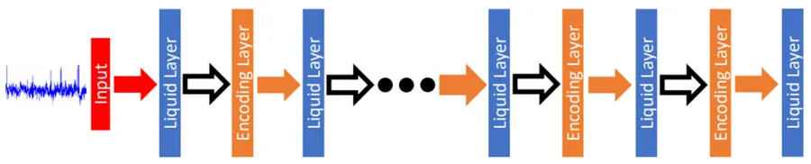Figure 4. A comparison of LNN performance vs. DNN’s in analyzing financial time series data

Trade-offs and Limitations

Computational Complexity

The dynamic nature of Liquid Neural Networks often requires more complex training procedures, such as Backpropagation Through Time (BPTT), which can be computationally intensive.

Stability Concerns

Managing the continuous state evolution poses challenges like vanishing or exploding gradients. Ensuring stability requires careful tuning of time constants and other hyperparameters.

Interpretability

While traditional networks are well-studied and understood, the dynamic behavior of liquid models can sometimes complicate the interpretation of how specific inputs influence the output over time.

Hybrid Approaches

In some scenarios, researchers combine static and liquid components to leverage the strengths of both architectures. These hybrid models aim to achieve the flexibility of liquid networks while retaining some of the simplicity and efficiency of traditional networks.

Figure 5. Comparison between traditional and liquid neural networks

This diagram contrasts the fixed nature of traditional networks with the dynamic properties of liquid models, emphasizing the key areas where they differ.

Summary

Liquid Neural Networks offer a powerful alternative to traditional static models by incorporating continuous adaptation and temporal dynamics. While they bring significant advantages in handling real-time and time-dependent data, they also introduce challenges in training complexity, stability, and interpretability. Understanding these trade-offs is essential when selecting the appropriate architecture for a given task.

Chapter 8: Future Directions and Open Research Questions

In this chapter, we explore emerging trends, potential improvements, and open research questions in the field of Liquid Neural Networks. As a dynamic and evolving area of study, liquid models offer promising opportunities as well as challenges that require further investigation.

Emerging Trends

Integration with Other Technologies

Researchers are exploring how Liquid Neural Networks can be integrated with other AI and machine learning paradigms, including:

• Reinforcement Learning: Combining liquid models with reinforcement learning to improve decision-making in dynamic environments.
• Neuromorphic Computing: Implementing liquid dynamics on hardware that mimics the neural architecture of the human brain, potentially leading to more efficient processing.

Scalability and Efficiency

A major focus is on scaling liquid models to handle large datasets and complex tasks without compromising the dynamic adaptation capabilities. Efforts include:

• Developing more efficient training algorithms.
• Optimizing the network architecture to reduce computational load.

Open Research Questions

Stability and Convergence

One significant area of inquiry is understanding how to maintain stability in continuously evolving networks. Questions include:

• What are the optimal settings for time constants $\tau$ that balance responsiveness with stability?
• How can we design training strategies to mitigate issues like vanishing or exploding gradients in continuous-time models?

A typical stability equation under investigation is:

Interpretability and Transparency

As liquid networks become more complex, understanding their decision-making process is crucial. Researchers are working on:

• Techniques for visualizing the evolution of internal states.
• Methods to explain how specific inputs affect the network’s dynamic behavior.

Generalization Across Domains

Another open question is how well liquid models generalize to different domains beyond time-series forecasting and control systems. Future work may explore:

• Applications in natural language processing, where context and sequence are vital.
• Cross-domain learning where a single model adapts to multiple types of dynamic data.

Interdisciplinary Collaboration

The development of Liquid Neural Networks is inherently interdisciplinary, involving:

• Mathematics: For the continuous-time modeling and differential equations.
• Computer Science: For algorithm development and computational optimization.
• Neuroscience: For insights into biological neural dynamics and adaptability.
• Engineering: For real-world applications in robotics and autonomous systems.

This collaboration can drive innovative solutions that bridge theoretical advances with practical implementations.

Chapter 9: Appendices and Supplementary Materials

This chapter provides additional resources to support your understanding of Liquid Neural Networks. It includes detailed mathematical derivations, code examples for implementation, a glossary of key terms, and recommendations for further reading.

Detailed Mathematical Derivations

For readers interested in a deeper dive into the mathematics behind Liquid Neural Networks, this section includes extended derivations. For example, a derivation of the continuous state update rule may begin with the basic differential equation:

A step-by-step derivation can explore:

• Separation of Variables: Techniques to solve the homogeneous part.
• Integration: Methods to integrate the inhomogeneous term.
• Stability Analysis: Insights into conditions ensuring convergence of $\mathbf{h}(t)$ .

These derivations provide the mathematical foundation for understanding how dynamic adaptation is achieved.

Code Examples and Implementation Guidelines

For practical application, a number of code examples are provided. These examples are intended to help you implement a basic Liquid Neural Network in popular frameworks such as TensorFlow or PyTorch. Below is a pseudo-code snippet illustrating the integration of dynamic state updates:

# Pseudo-code for a dynamic state update in a Liquid Neural Network
def liquid_state_update(h, x, W, U, b, tau, dt):
    # Compute the derivative of the state using the differential equation
    dh_dt = - (1 / tau) * h + activation(np.dot(W, h) + np.dot(U, x) + b)
    
    # Update state using Euler's method
    h_next = h + dh_dt * dt
    
    return h_next

# Example usage:
# h: current state vector
# x: current input vector
# W, U: weight matrices
# b: bias vector
# tau: time constant
# dt: time step for integration

These guidelines aim to provide a starting point for experimentation and further customization.

Glossary of Key Terms

• Liquid Neural Network (LNN): A neural network that continuously adapts its internal state over time using differential equations.
• Deep Neural Network (DNN): A neural network with multiple layers and fixed parameters during inference.
• Time Constant ($\tau$ ): A parameter that controls the speed of state evolution in a dynamic system.
• Activation Function ($\sigma$ ): A nonlinear function applied to the output of neurons to introduce nonlinearity.
• Backpropagation Through Time (BPTT): An extension of the backpropagation algorithm used for training networks with temporal dependencies.
• Euler’s Method: A numerical technique for solving ordinary differential equations.

Recommended Further Reading

For readers who wish to delve even deeper into the topics covered in this primer, consider exploring the following:

• Research articles on continuous-time neural networks and their applications.
• Textbooks on dynamical systems and differential equations.
• Online tutorials and courses focusing on advanced neural network architectures.