Kolmogorov-Arnold Neural Networks

Introduction

In the rapidly evolving landscape of artificial intelligence, neural networks have emerged as a cornerstone, driving advancements in machine learning, data analysis, and automation. Among the myriad architectures proposed, the Kolmogorov-Arnold Neural Network (KANN) stands out, offering a unique approach rooted in rigorous mathematical theory. While the prevailing models like convolutional and recurrent neural networks have garnered widespread acclaim for their performance across various tasks, KANNs present a compelling alternative that merits closer examination.

The foundation of KANNs is anchored in the pioneering work of Andrey Kolmogorov and Vladimir Arnold, who formulated the superposition theorem and its extensions. This theorem posits that any continuous multivariate function can be represented as a finite composition of continuous functions of a single variable and addition. Such a theoretical underpinning holds profound implications for the design and functionality of neural networks, promising enhanced representation capabilities and potentially more efficient training paradigms.

Despite their theoretical elegance, Kolmogorov-Arnold neural networks have not yet enjoyed the same level of practical application and recognition as their more conventional counterparts. This paper seeks to bridge this gap by elucidating the architecture, training methods, and potential applications of KANNs. Through rigorous analysis and experimental validation, we aim to showcase the strengths and address the limitations of this intriguing neural network model.

In an era where the capabilities of artificial intelligence are expanding at an unprecedented rate, understanding and leveraging the full spectrum of available neural network architectures is crucial. By delving into the nuances of KANNs, we contribute to a broader comprehension of neural networks and open new avenues for research and application. The subsequent sections will unpack the theoretical foundations, architectural details, and practical implementations of Kolmogorov-Arnold neural networks, offering insights that could pave the way for future innovations in the field.

Theoretical Foundation

Kolmogorov-Arnold Superposition Theorem

The Kolmogorov-Arnold superposition theorem is a pivotal result in the field of functional analysis. It states that any continuous function f : [0,1]^n → ℝ can be represented as a finite composition of continuous functions of one variable and addition. Specifically, for any continuous function f, there exist continuous functions φ_i : ℝ → ℝ and ψ_i : ℝ → ℝ such that:

Here, $\phi_{ij}$ and $\psi_i$ are continuous functions that transform the input variables $x_j$ into a sum that is then mapped by the $\psi_i$ functions.

Arnold’s Extension

Building on Kolmogorov’s theorem, Vladimir Arnold extended this concept, showing that the number of required inner functions can be reduced under certain conditions. Arnold demonstrated that it is possible to represent f using:

This reduction significantly impacts the practical implementation by decreasing the computational complexity and the number of components required.

Examples

Kolmogorov-Arnold Superposition Theorem

Example 1:

Input:

Consider a simple continuous function $f(x_1, x_2) = x_1^2 + x_2^2$ .

Steps:

Identify Component Functions: According to the theorem, we need to find continuous functions $\phi_{ij}$ and $\psi_i$ such that the function can be decomposed.

Decomposition:

Choosing φ and ψ:

Substitute Back:

Output:

The function is successfully decomposed as a sum of continuous functions of one variable.

Example 2:

Input:

Consider the continuous function $f(x_1, x_2) = e^{x_1} \cdot \sin(x_2)$ .

Steps:

Identify Component Functions: According to the theorem, we need to find continuous functions $\phi_{ij}$ and $\psi_i$ such that the function can be decomposed.

Decomposition:

Choosing φ and ψ:

Substitute Back:

Output:

The function is successfully decomposed as a sum of continuous functions of one variable.

B-Splines

B-splines, or basis splines, are piecewise-defined polynomials used in approximation theory and data fitting. They provide a versatile tool for function representation and interpolation. The theory behind B-splines involves constructing a series of polynomial segments joined at specific points called knots.

Definition and Properties

A B-spline of degree k is defined recursively. The zeroth-degree B-spline, $B_i^0(t)$ , is defined as:

For k > 0, the B-spline $B_i^k(t)$ is defined as:

Here, $t_i$ are the knots that determine where each polynomial segment begins and ends. A knot is a point that defines the intervals over which the polynomial segments are defined and joined together.

What are knots?

Knots are specific values in the input domain where the pieces of the polynomial functions meet. They essentially define the intervals over which the polynomial segments are defined and joined together.

Think of knots as points on the x-axis where you can transition from one polynomial piece to another. In practical terms, knots help to determine where the influence of a given control point or segment of the polynomial begins and ends.

How do we decide what values we choose for the knots?

The values for a knot sequence in B-splines can be chosen based on several factors, including the domain of the data, the desired smoothness of the resulting spline, and the specific requirements of the application. Here are some common methods and considerations for determining knot values:

1. Uniform Knot Sequence

In a uniform knot sequence, the knots are evenly spaced. This is the simplest approach and is often used for equally spaced data points.

Example:

For 6 data points, you might choose a uniform knot sequence like:

t=[0, 1, 2, 3, 4, 5]

2. Non-Uniform Knot Sequence

In a non-uniform knot sequence, the knots can be spaced irregularly. This approach allows more flexibility and can be used to give more control points influence over specific regions of the curve.

Example:

If you have data points that are not evenly spaced, you might choose a knot sequence like:

t = [0, 0.5, 1.5, 2.5, 4, 5]

3. Clamped or Open Knot Sequence

A clamped or open knot sequence repeats the first and last knots to ensure that the B-spline starts and ends at the first and last control points. This is useful for creating splines that touch the boundary points.

Example:

For a cubic B-spline with 4 control points, you might choose:

t=[0, 0, 0, 1, 2, 3, 3, 3]

Steps to Determine Knot Values

1. Determine the Degree of the B-Spline: The degree k of the B-spline influences the number of knots and the smoothness of the spline. Common choices are linear (degree 1), quadratic (degree 2), and cubic (degree 3).

2. Count the Control Points: Let n be the number of control points. The total number of knots required is n+k+1

3. Choose the Knot Values:

   • Uniform Knots: Space the knots evenly over the domain.

   • Non-Uniform Knots: Place knots based on the distribution of data points or specific requirements.

   • Clamped/Open Knots: Repeat the first and last knots k times for a degree k B-spline.

What are B-spline control points?

Control points are the key components in defining the shape and properties of a B-spline curve. They act as reference points that influence the curve, but the curve does not necessarily pass through them. Here is an explanation of control points, their role, and how they interact with B-splines.

Control Points Explained

Definition

Control points are a set of points that determine the shape of the B-spline curve. Each control point has a coordinate in the space in which the curve is defined, typically denoted as $P_i = (x_i, y_i)$ in 2D or $P_i = (x_i, y_i, z_i) \text{ in 3D}$ .

Role in B-Splines

1. Influence on Curve Shape: The position of each control point affects the shape of the B-spline curve. The curve is “pulled” towards each control point but does not necessarily pass through it, allowing for smooth and flexible shapes.

2. Local Control: Moving a single control point affects only a portion of the B-spline curve, providing local control over the curve’s shape. This property is useful for fine-tuning specific segments without altering the entire curve.

3. Weighted Influence: Each control point has an associated basis function that defines its influence over the curve. The combination of these basis functions, determined by the knot sequence and degree of the spline, forms the final shape of the curve.

Mathematical Representation

A B-spline curve of degree k with n control points is defined as:

Where:

• C(t) is the B-spline curve.

• $N_{i,k}(t)$ are the B-spline basis functions of degree k.

• $P_i$ are the control points.

Example: Cubic B-Spline with Control Points

Let’s consider a cubic B-spline (k = 3) with four control points:

Control Points:

Knot Sequence:

B-Spline Basis Functions for Cubic B-Spline (k = 3):

For the interval [0, 1]:

The B-spline curve C(t) is then given by:

By substituting the values of the control points and the basis functions, you can compute the specific points on the B-spline curve.

Example: Cubic B-Spline with 4 Control Points

Degree k=3

Number of Control Points n=4

Total Number of Knots:

Uniform Knot Sequence:

Clamped/Open Knot Sequence:

Summary

• Uniform Knots: Evenly spaced, simple to implement.

• Non-Uniform Knots: Irregularly spaced, more flexible.

• Clamped/Open Knots: Repeated first and last knots for boundary constraints.

The choice of knot values affects the shape and flexibility of the B-spline. Uniform knots are simpler but less flexible, while non-uniform and clamped knots provide more control over the spline’s shape.

B-Splines

Example 1:

Input:

Consider the knots $t = [0, 1, 2, 3, 4, 5]$ and we want to construct a B-spline of degree 2.

Steps:

Define Zeroth-Degree B-Splines:

and so on

First-Degree B-Splines:

and so on

Second-Degree B-Splines:

and so on

Output:

The B-splines of degree 2 constructed for the given knots.

Example 2:

Input:

Consider the knots $t = [0, 1, 2, 3, 4]$ and we want to construct a B-spline of degree 3.

Steps:

Define Zeroth-Degree B-Splines:

and so on

First-Degree B-Splines:

and so on

Second-Degree B-Splines:

and so on

Third-Degree B-Splines:

and so on

Output:

The B-splines of degree 3 constructed for the given knots.

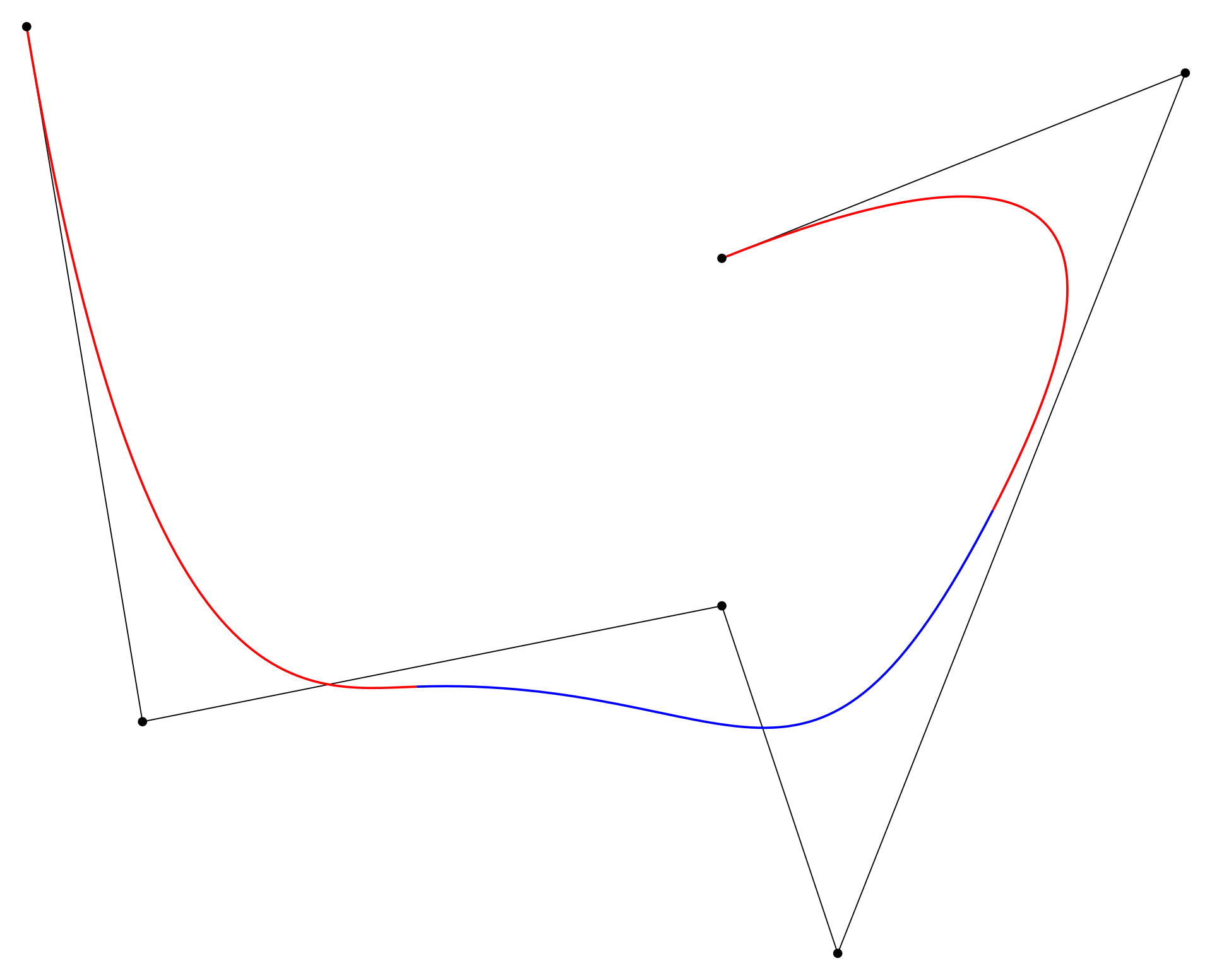
Diagram 1. A visual example of B-splines

Kolmogorov-Arnold Neural Networks (KANNs)

Kolmogorov-Arnold Neural Networks (KANNs) are a class of neural networks inspired by the Kolmogorov-Arnold representation theorem. This theorem states that any multivariate continuous function can be represented as a superposition of continuous functions of one variable and addition. KANNs utilize this theoretical foundation along with practical function approximation methods like B-splines to create powerful neural network models.

Structure of KANNs

Input Layer: Contains (n) nodes corresponding to the (n) input variables.

Hidden Layers: Perform transformations using functions ($\phi_{ij}$ ). These layers can be implemented using B-splines to approximate these functions.

Output Layer: Combines the outputs of the hidden layers using functions ($\psi_i$ ), again using B-splines for smooth approximation.

Working of KANNs

Transformation by Hidden Layers: Each hidden layer transforms the input variables through functions ($\phi_{ij}(x_j)$ ), which can be represented by B-splines:

Combination by Output Layer: The output layer applies functions ($\psi_i$ ) to these kannte representations and sums them up to produce the final output:

Example of KANN

Let’s consider a simple example where we have a 2-dimensional input vector ( $(x_1, x_2)$ ) and we want to approximate a function ( $f(x_1, x_2)$ ).

Input Layer: Two input nodes for ( $x_1$ ) and ( $x_2$ ).

Hidden Layer Transformation:

Suppose we have 3 hidden nodes, and each node uses a B-spline to transform the inputs:

Here, each ( $\phi_{ij}$ ) is a B-spline function approximating a univariate function of ( $x_1$ ) or ( $x_2$ ).

Output Layer Combination:

The output layer combines these hidden representations using additional B-spline functions:

Handling High-Dimensional Input with KANNs

Kolmogorov-Arnold Neural Networks (KANNs) have a theoretical foundation that allows them to approximate any continuous multivariate function, which includes functions with a large number of input variables. However, the practical implementation and efficiency of KANNs in handling high-dimensional inputs depend on several factors.

Theoretical Capability

The Kolmogorov-Arnold representation theorem ensures that any continuous function of ( n ) variables can be decomposed into sums of continuous functions of one variable. This means that, in theory, KANNs can handle functions with a large number of input variables.

Practical Considerations

While the theoretical foundation is robust, practical challenges arise when dealing with high-dimensional inputs:

Number of Hidden Units: According to the theorem, the number of hidden units required is typically ( 2n + 1 ), where ( n ) is the number of input variables. For high-dimensional inputs, this results in a large number of hidden units, which can increase the complexity of the network.

Parameter Explosion: As the number of input variables increases, the number of parameters (e.g., B-spline coefficients) in the network also increases. This can lead to high memory requirements and longer training times.

Training Complexity: Training a network with many parameters requires a large amount of data to avoid overfitting and to ensure that the model generalizes well. High-dimensional data often requires sophisticated techniques for efficient training.

Computational Resources: Handling high-dimensional inputs necessitates significant computational resources, both in terms of processing power and memory.

Mitigation Strategies

To address these challenges, several strategies can be employed:

Dimensionality Reduction: Techniques such as Principal Component Analysis (PCA), t-SNE, or autoencoders can be used to reduce the dimensionality of the input data before feeding it into the network.

Regularization: Regularization techniques such as L1/L2 regularization, dropout, and weight sharing can help mitigate overfitting and manage the complexity of the model.

Efficient Representations: Using more efficient representations of ( $\phi_{ij}$ ) and ( $\psi_i$ ) functions can reduce the number of parameters. For example, piecewise linear functions or lower-degree B-splines might offer a trade-off between complexity and approximation capability.

Parallel and Distributed Computing: Leveraging parallel and distributed computing frameworks can help manage the computational load associated with training large KANNs.

Sparse Representations: Employing sparse representations of the input data can help reduce the effective dimensionality and improve computational efficiency.

Example with High-Dimensional Input

Suppose we have a function (f) with 100 input variables ($x_1, x_2, \ldots, x_{100}$ ). According to the Kolmogorov-Arnold theorem, we would need at least (201) hidden units:

Input Layer: 100 input nodes for ( $x_1, x_2, \ldots, x_{100}$ ).

Hidden Layer Transformation:

Each hidden unit performs a transformation using B-splines:

Here, each ( $\phi_{ij}$ ) is a B-spline function approximating a univariate function of ( $x_j$ ).

Output Layer Combination:

The output layer combines these hidden representations using additional B-spline functions:

While KANNs have the theoretical capability to handle high-dimensional inputs, practical implementations must address the challenges of parameter explosion, training complexity, and computational resource requirements. By employing dimensionality reduction, regularization, efficient representations, and leveraging advanced computational techniques, KANNs can be made more practical for high-dimensional function approximation tasks.

Diagram 2. A comparison of MLPs vs. KANNs

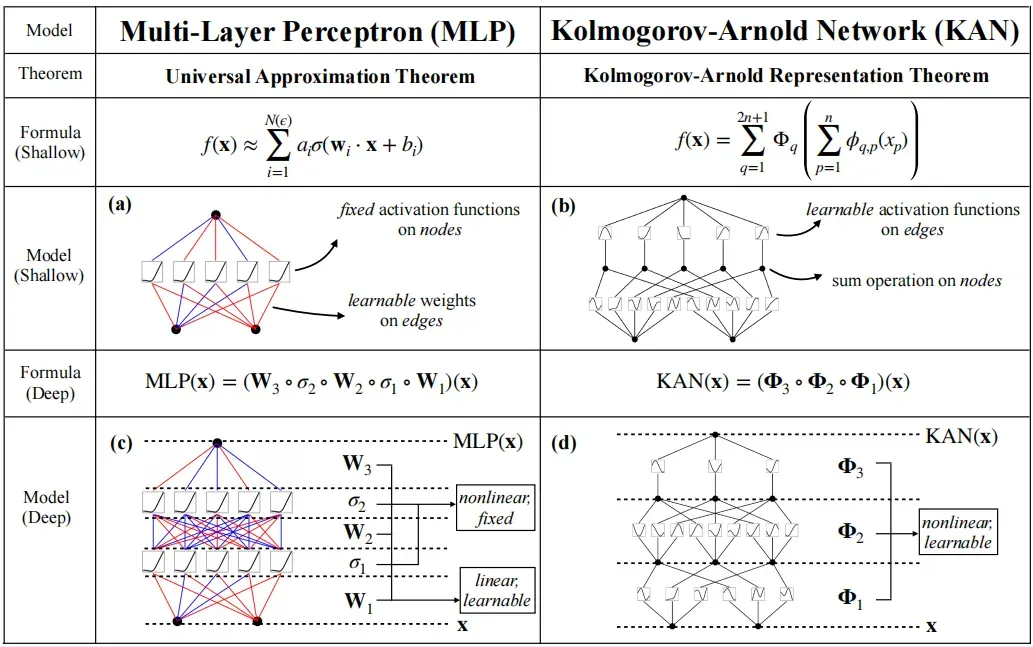
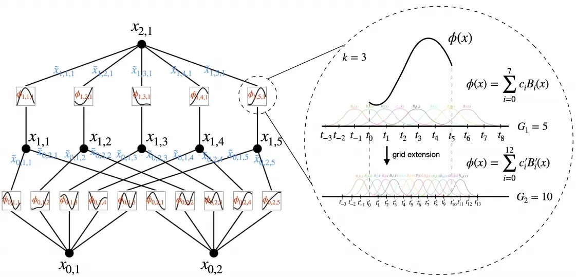
Diagram 3. A pictorial representation of KANNS. Note the input vector members being fed into activation functions rather than assigned static weights.

B-Splines and KANNs

B-splines (Basis splines) are often used in conjunction with Kernel-based Artificial Neural Networks (KANNs) due to their advantageous properties for approximating complex functions and improving the learning process. Here are some reasons and advantages for using B-splines with KANNs:

Smoothness and Flexibility

Reason:

• B-splines provide a smooth and flexible way to approximate complex, non-linear functions. They are defined piecewise by polynomial functions, which can be easily adjusted to fit various shapes and data trends.

• Advantage:

• This smoothness ensures that the approximated functions are continuous and differentiable, which is crucial for tasks that require gradient-based optimization methods, such as backpropagation in neural networks.

Local Control

Reason:

• B-splines have local support, meaning that adjusting a control point affects the function only in a local region around that point.

Advantage:

• This property is beneficial in neural networks because it allows for localized adjustments without impacting the entire function, leading to more stable and efficient learning processes. It also makes the model more interpretable and easier to debug.

Reduced Overfitting

Reason:

• B-splines can be used to construct smooth approximations with fewer parameters compared to other basis functions.

Advantage:

• By using fewer parameters to achieve a smooth fit, B-splines help in reducing the risk of overfitting, which is particularly important in machine learning where overfitting to the training data can lead to poor generalization on unseen data.

Computational Efficiency

Reason:

• The piecewise polynomial nature of B-splines allows for efficient computation of function values and their derivatives.

Advantage:

• This efficiency is crucial for training neural networks, especially for large-scale problems or when using deep architectures, as it reduces the computational burden and speeds up the training process.

Robustness to Noise

Reason:

• B-splines can smooth out noise in the data due to their inherent smoothing properties.

Advantage:

• This robustness makes KANNs with B-splines more effective in handling real-world data, which is often noisy and imperfect, leading to better performance and more reliable models.

Versatility in High Dimensions

Reason:

• B-splines can be extended to higher dimensions using tensor product splines.

Advantage:

• This versatility allows KANNs to handle multi-dimensional data more effectively, making them suitable for complex tasks such as image processing, time-series analysis, and other applications involving high-dimensional inputs.

Sparse Representations in KANNs

Sparse representations of input data can significantly improve the computational efficiency of Kolmogorov-Arnold Neural Networks (KANNs) by reducing the effective dimensionality and the amount of computation required. Here’s how they can help:

Understanding Sparse Representations

A sparse representation means that most of the elements in the input data vector are zero. This can happen naturally in many applications, such as text data (bag-of-words models), image data (where most pixels might be background), or sensor data (where only a few sensors are active at any given time).

Benefits of Sparse Representations

Reduced Computational Load: When many input features are zero, the network can skip computations involving those features, saving time and resources.

Memory Efficiency: Sparse data can be stored more efficiently using data structures like sparse matrices, which only store non-zero elements and their indices.

Faster Training: With fewer active features, the number of parameters that need to be updated during training is reduced, leading to faster convergence.

Regularization Effect: Sparsity can act as a form of regularization, potentially improving the generalization of the model by reducing the risk of overfitting.

Implementing Sparse Representations in KANNs

Here’s how sparse representations can be leveraged in KANNs:

Sparse Input Layer: Use data structures optimized for sparse data, such as sparse matrices or tensors. This ensures that only non-zero elements contribute to the computations.

Efficient Computation in Hidden Layers:

Sparse Matrix Operations: Use libraries and frameworks that support sparse matrix operations. In many machine learning libraries, operations on sparse matrices are optimized to skip zero elements.

Activation Functions: Ensure that the activation functions and B-spline transformations in the hidden layers are implemented to handle sparse inputs efficiently.

Sparse B-Spline Representations: If the functions $\phi_{ij}$ and $\psi_i$ can be represented using sparse B-splines, this can further reduce the number of parameters and computations. Sparse B-splines only store and compute the non-zero coefficients.

Training with Sparse Data: When training with sparse data, gradient updates can be computed more efficiently by focusing only on the non-zero elements. This reduces the number of weight updates needed per training iteration.

Example of Sparse Computation

Consider a KANN with an input vector (x) of dimension 1000, where only 10 elements are non-zero. The hidden layers use B-splines to transform the inputs, and the output layer combines these transformations.

Sparse Input Representation:

import numpy as np
from scipy.sparse import csr_matrix

# Sparse input vector
x_sparse = csr_matrix((data, indices, indptr), shape=(1, 1000))
Sparse Matrix Operations:

# Sparse matrix multiplication with weights
hidden_layer_output = x_sparse.dot(weight_matrix)

# Sparse input vector
x_sparse = csr_matrix((data, indices, indptr), shape=(1, 1000))

Sparse B-Spline Transformation:

# Assuming B-spline transformations are implemented to handle sparse inputs
transformed_output = sparse_b_spline_transform(hidden_layer_output)

# Sparse Gradient Updates:
# Compute gradients only for non-zero elements
gradients = compute_gradients(transformed_output, target)

Sparse representations can greatly enhance the computational efficiency of KANNs by reducing the effective dimensionality of the input data and focusing computational resources on the relevant (non-zero) elements. By integrating sparse data structures and optimized operations, KANNs can handle high-dimensional inputs more efficiently, making them more practical for real-world applications involving large and sparse datasets.

Implementing Sparse Representations to Reduce Overfitting

To effectively leverage sparse representations for reducing overfitting in KANNs, consider the following strategies:

Sparse Input Handling:

Use data structures and libraries optimized for sparse data (e.g., scipy.sparse in Python) to efficiently handle and process sparse inputs.

Ensure the input layer of the KANN is designed to work with sparse data, skipping computations for zero elements.

Regularization Techniques:

Combine sparse representations with traditional regularization methods like L1 and L2 regularization to further constrain the model complexity.

Use dropout, which randomly zeros out parts of the input data or kannte representations during training, to promote sparsity and reduce overfitting.

Sparse B-Splines:

Implement B-spline functions that can operate on sparse inputs, focusing on non-zero coefficients to maintain sparsity throughout the network.

Data Preprocessing:

Apply techniques such as feature selection or dimensionality reduction to preprocess the data, ensuring that only the most relevant features are retained and represented sparsely.

Example Workflow

Here’s an example of how you might implement these strategies in practice:

Sparse Data Representation:

from scipy.sparse import csr_matrix
from sklearn.linear_model import Lasso
import tensorflow as tf

# Create a sparse matrix from input data
x_sparse = csr_matrix((data, indices, indptr), shape=(n_samples, n_features))

# Perform sparse matrix multiplication
hidden_layer_output = x_sparse.dot(weight_matrix)

# Perform sparse matrix multiplication
hidden_layer_output = x_sparse.dot(weight_matrix)

# Apply L1 regularization to promote sparsity
lasso = Lasso(alpha=0.1)
lasso.fit(x_sparse, y)

# Apply dropout to the hidden layer
dropout_layer = tf.keras.layers.Dropout(rate=0.5)
hidden_layer_output = dropout_layer(hidden_layer_output, training=True)

By incorporating these techniques, you can leverage sparse representations to build more robust KANNs that generalize better and are less prone to overfitting.

Appendix A: Splines

A spline is a mathematical function used for interpolation or smoothing of data points. It is a piecewise-defined polynomial function that ensures smoothness at the places where the polynomial pieces connect, known as “knots”. Splines are widely used in various fields such as computer graphics, data fitting, and numerical analysis due to their flexibility and ability to create smooth curves through a given set of points.

Key Characteristics of Splines

Piecewise Polynomials: Splines are composed of several polynomial segments. Each segment is defined over a specific interval, and the collection of these segments forms the entire spline function.

Knots: The points where the polynomial segments meet are called knots. The placement and number of knots can significantly affect the shape and properties of the spline.

Continuity: Splines are typically designed to be continuous up to a certain degree of derivatives at the knots. For example, a cubic spline not only ensures the function itself is continuous but also its first and second derivatives are continuous at each knot.

Degree: The degree of the polynomial pieces can vary. Common types of splines include:

Linear splines: Piecewise linear functions.

Quadratic splines: Piecewise quadratic functions.

Cubic splines: Piecewise cubic functions, often used due to their balance between flexibility and computational efficiency.

Types of Splines

Linear Splines: These are the simplest form, where each segment is a linear function. They are not smooth as they have discontinuities in their first derivatives at the knots.

Quadratic Splines: These use quadratic polynomials for each segment. They ensure continuity of the function and its first derivative.

Cubic Splines: These are the most commonly used splines. They use cubic polynomials for each segment, ensuring continuity of the function and its first and second derivatives. Cubic splines are widely used because they provide a good balance between smoothness and computational simplicity.

B-Splines: These are a generalization of splines that use basis functions. B-splines provide local control over the shape of the curve, meaning that changing a control point affects only a local portion of the spline.

NURBS (Non-Uniform Rational B-Splines): These extend B-splines by adding weights to the control points, allowing for the representation of more complex shapes, including conic sections and freeform surfaces.

Applications of Splines

Data Fitting: Splines are used to fit smooth curves to a set of data points. This is useful in statistics, machine learning, and other fields where modeling and analyzing data trends are essential.

Computer Graphics: In graphics and CAD (Computer-Aided Design), splines are used to design smooth and flexible curves and surfaces. B-splines and NURBS are particularly popular in these applications.

Numerical Analysis: Splines are used in numerical solutions of differential equations, where they can approximate solutions with high accuracy.

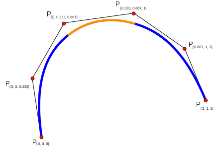
Diagram 4. Example of a spline function with single knots at 1/3 and 2/3.

Appendix B. Differences between generic splines and B-splines.

Splines and B-splines are both used in numerical analysis and computer graphics to create smooth curves through a set of points. However, they have distinct differences in their definitions, properties, and applications. Below, we explore these differences in detail.

Splines

Splines refer to a broad category of piecewise polynomial functions that can be used to approximate or interpolate data points. The term “spline” originally comes from the flexible strips used by draftsmen to draw smooth curves through a set of points. In mathematics and computer science, splines are defined more formally as follows:

Piecewise Polynomial: Splines are composed of polynomial segments joined at certain points called “knots”.

Continuity: Splines typically have a specified degree of smoothness at the knots. For example, a cubic spline (made up of third-degree polynomials) is usually required to have continuous first and second derivatives at the knots.

Types: There are various types of splines, including linear, quadratic, and cubic splines, depending on the degree of the polynomial.

B-splines

B-splines (Basis splines) are a specific type of spline with additional properties that make them particularly useful in computer graphics and numerical analysis:

Basis Functions: B-splines are defined by a set of basis functions, which are piecewise polynomials of a given degree. These basis functions have local support, meaning they are non-zero over only a small portion of the domain.

Local Control: Because each basis function affects only a limited portion of the curve, B-splines offer local control over the shape of the spline. Modifying a control point influences only the nearby segments of the curve.

Knot Vector: B-splines require a knot vector, which is a non-decreasing sequence of parameter values that determine where and how the basis functions are defined. The repetition of knots can affect the continuity and smoothness at those points.

Types of B-splines: By adjusting the knot vector and the degree of the polynomials, you can create various types of B-splines, such as uniform B-splines (with evenly spaced knots) or non-uniform B-splines.

NURBS: Non-Uniform Rational B-Splines (NURBS) are an extension of B-splines that include weights for each control point, allowing for the representation of more complex shapes, including conic sections.

Key Differences

General vs. Specific: Splines are a general concept, while B-splines are a specific type of spline with well-defined basis functions and properties.

Basis Functions: B-splines are constructed using basis functions, which provide local control over the spline. General splines do not necessarily have this property.

Local Control: B-splines offer local control due to their basis functions with local support. Adjusting a control point in a B-spline affects only a portion of the curve, whereas in general splines, adjusting a control point might influence the entire curve.

Knot Vector: B-splines require a knot vector to define the piecewise polynomial segments, whereas general splines might not explicitly use a knot vector.

Applications

Splines: General splines are used in interpolation, approximation, and smoothing of data. Applications include numerical analysis, data fitting, and computer graphics.

B-splines: B-splines are widely used in computer-aided design (CAD), computer graphics, and animation for creating smooth and flexible shapes. They are also used in numerical solutions of differential equations and other areas where local control of the spline is advantageous.

Conclusion

In summary, while both splines and B-splines are used to create smooth curves, B-splines provide additional structure and properties that make them particularly useful for applications requiring local control and flexibility. Understanding these differences helps in choosing the appropriate type of spline for a given application.