AI Weekly Report Briefing

By AI Research Team

Hamiltonian and Lagrange Neural Networks

Introduction

Hamiltonian and Lagrange neural networks represent a sophisticated integration of classical mechanics with modern neural network architectures. These frameworks are particularly useful for modeling physical systems and dynamical processes, leveraging the principles of Hamiltonian and Lagrangian mechanics to improve the learning capabilities and interpretability of neural networks.

You can view the Jupyter Notebook for this briefing

Primer on Hamiltonian and Lagrangian Mechanics

Hamiltonian Mechanics

Hamiltonian mechanics is a reformulation of classical mechanics introduced by William Hamilton in the 19th century. It provides a powerful and elegant way to describe the evolution of physical systems over time, especially those with conserved quantities like energy, momentum, and angular momentum.

Why Hamiltonian Equations are Useful:

Conservation Laws: They inherently conserve energy, momentum, and other physical quantities.
Symplectic Structure: They preserve the geometric structure of phase space, ensuring accurate long-term predictions.
Applicability: They are versatile, applicable to a wide range of physical systems, including those with complex interactions.
Predictive Power: They offer precise predictions of system behavior over time

Hamiltonian Function

The Hamiltonian $H$ is a function of generalized coordinates $q$ and conjugate momenta $p$ , often representing the total energy of the system:

H(q,p) = T(p) + V(q)

where $T(p)$ is the kinetic energy and $V(q)$ is the potential energy. Physicists use the Hamiltonian function because it provides a comprehensive description of the system’s energy, combining both kinetic and potential components.

Hamilton’s Equation

The dynamics of the system are described by Hamilton’s equations, which are first-order differential equations:

\dot{q} = \frac{\partial H}{\partial p}, \quad \dot{p} = -\frac{\partial H}{\partial q}

These equations describe how the state of the system evolves over time. Physicists use Hamilton’s equations because they offer a systematic way to analyze the motion of a system, particularly when dealing with complex interactions and multiple degrees of freedom.

Hamiltonian equations are used in a number of areas, including:

Celestial Mechanics: Used in astrophysics to predict the orbits of planets, stars, and satellites.
Quantum Mechanics: Fundamental in quantum mechanics to describe the total energy of a quantum system.
Control Systems: Applied in engineering to design and analyze control systems that need to conserve energy.

Lagrangian Mechanics

Lagrangian mechanics, another formulation of classical mechanics, uses the Lagrangian function to describe the dynamics of a system in terms of generalized coordinates $q$ and generalized velocities $\dot{q}$ .

This approach is particularly powerful for systems with constraints and provides a framework for deriving the equations of motion without directly solving Newton’s second law.

Lagrangian Function

The Lagrangian $L$ is defined as the difference between the kinetic and potential energy of the system:

L(q, \dot{q}) = T(\dot{q}) - V(q)

Lagrangian equations are fundamental in classical mechanics and provide an alternative formulation to Newton’s laws. They offer several advantages:

Simplification of Complex Systems: Lagrangian mechanics often simplifies the analysis of systems with constraints (e.g., pendulums, robotic arms).
Generalized Coordinates: It uses generalized coordinates, making it easier to describe the system’s configuration.
Derivation of Equations of Motion: The Euler-Lagrange equations derived from the Lagrangian function simplify obtaining the equations of motion for complex systems.

Euler-Lagrange Equations

The Euler-Lagrange equations are a set of second-order differential equations that provide the equations of motion for a system described by a Lagrangian function. They are derived from the principle of least action, which states that the actual path taken by a system is the one that minimizes the action S, defined as the integral of the Lagrangian L over time.

For a system with generalized coordinates q and generalized velocities $\dot{q}$ , the Euler-Lagrange equation is:

\frac{d}{dt} \left( \frac{\partial L}{\partial \dot{q}} \right) - \frac{\partial L}{\partial q} = 0

These equations of motion are derived from the Euler-Lagrange equations, which are second-order differential equations. These equations describe how the generalized coordinates evolve over time.

The differences from the Lagrangian Equations are:

Lagrangian: The Lagrangian L is a function that combines the kinetic energy T and potential energy V of the system: L = T - V.
Euler-Lagrange Equations: These are derived from the Lagrangian and provide the equations of motion for the system.

Advantages:

Handles Constraints: The Euler-Lagrange equations are particularly powerful for dealing with systems that have constraints, such as pendulums or robotic arms.
Generalized Coordinates: They allow the use of generalized coordinates, which can simplify the analysis of complex systems.

Example:

For a simple pendulum, the Lagrangian is:

L = T - V = \frac{1}{2} ml^2 \dot{\theta}^2 - mgl(1 - \cos \theta)

The Euler-Lagrange equation for this system is:

\frac{d}{dt} (ml^2 \dot{\theta}) + mgl \sin \theta = 0

This provides the equation of motion for the pendulum in terms of the angle $\theta$ .

Real-World Use Cases:

Robotics: Used to model and control robotic systems, ensuring precise movements.
Biomechanics: Helps in understanding human movement dynamics and designing prosthetics.
Mechanical Engineering: Aids in analyzing and designing mechanical systems with constraints, such as linkages and suspension systems.

Invariants in Hamiltonian and Lagrangian Mechanics

Invariants are properties or quantities in a system that remain constant over time, no matter how the system evolves. Think of them as fixed landmarks in a changing landscape.

Why Invariants Matter:

Energy Conservation: Just like how the total amount of water in a closed system stays the same, the total energy in a physical system (kinetic + potential) remains constant.
Momentum Conservation: Imagine you’re in a smooth ice rink; if you push off and glide, your momentum (mass times velocity) remains unchanged until you hit something.
Angular Momentum: If you’re spinning in a swivel chair with your arms out and then pull them in, you spin faster. This is because your angular momentum is conserved.

In the context of Hamiltonian and Lagrangian mechanics, these invariants help ensure that the models we use to describe physical systems are accurate and stable over time.

Hamiltonian Neural Networks (HNNs)

Overview

Hamiltonian neural networks (HNNs) incorporate the principles of Hamiltonian mechanics into neural network architectures to model the dynamics of physical systems. By construction, these models learn conservation laws from data, leading to better performance in physics-based problems.

Learning the Hamiltonian Function

HNNs parameterize the Hamiltonian function $H(q,p)$ using neural network parameters and learn it directly from data. The learned Hamiltonian is used to predict the system’s evolution by adhering to Hamilton’s equations.

Incorporating Invariants

Energy Conservation: By learning a Hamiltonian function that remains invariant over time, HNNs ensure that the total energy of the system is conserved.
Symplectic Structure: The loss function in HNNs is designed to respect the symplectic structure, preserving the phase space volume and ensuring accurate long-term predictions.

Zero Divergence Property

The HNN learns a vector field that has zero divergence. In simple terms, when the Hamiltonian Neural Network (HNN) learns a vector field with zero divergence, it means that there are no points in the system where things are being added (sources) or removed (sinks). This property ensures that if we move the system forward in time and then backward, we end up exactly where we started. This makes the model very accurate and reliable over long periods, as it faithfully preserves the system’s state without distortion.

Loss Function

The loss function ensures that the learned Hamiltonian respects the symplectic structure, minimizing the discrepancy between the predicted and true dynamics.

In simple terms, a symplectic structure is a special way of organizing and preserving the information about a system’s state over time. Imagine you have a room full of balloons, each representing a possible state of the system. A symplectic structure ensures that as the system evolves, the overall arrangement and volume of the balloons don’t change, even though individual balloons might move around. This helps in accurately predicting the system’s behavior without losing or distorting any information.

The objective is to make the following terms go to zero:

\operatorname*{argmin}_\theta \bigg \Vert \frac{d\mathbf{q}}{dt} - \frac{\partial \mathcal{H}_{\theta}}{\partial \mathbf{p}} \bigg \Vert^2 ~+~ \bigg \Vert \frac{d\mathbf{p}}{dt} + \frac{\partial \mathcal{H}_{\theta}}{\partial \mathbf{q}} \bigg \Vert^2

Architecture

HNNs typically use a feedforward neural network to approximate the Hamiltonian function. Inputs are the generalized coordinates $q$ and momenta $p$ .

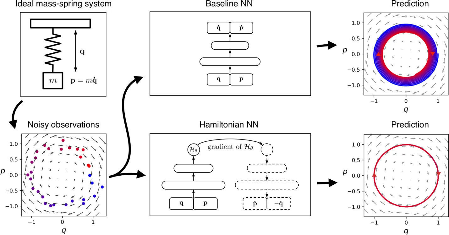Figure 1. A contrast between a standard neural network and a Hamiltonian neural network

In the above diagram we see that the Hamiltonian neural network evaluates its parameters via data. Beause the Haniltonian equation conserves quantities, it produces a much more robust and accurate prediction state. (Ref. https://greydanus.github.io/2019/05/15/hamiltonian-nns/)

Applications:

Celestial Mechanics: Modeling planetary orbits and satellite dynamics.
Particle Physics: Simulating interactions at a subatomic level.
Control Systems: Designing systems that need to maintain energy conservation over time.

Advantages Over Ordinary Deep Neural Networks

Preservation of Physical Laws: HNNs inherently preserve the conservation laws (e.g., energy) of the systems they model, which is crucial for long-term predictions.
Improved Generalization: By embedding physical principles into the learning process, HNNs generalize better to unseen data, especially in physical systems where these principles apply.
Enhanced Interpretability: The learned Hamiltonian function has a clear physical meaning, making the model’s predictions more interpretable in the context of the system’s dynamics.

Mass-Spring Example

The mass-spring system is a classic example in physics that illustrates how Hamiltonian mechanics can be used to describe the dynamics of a simple harmonic oscillator. Consider a mass $m$ attached to a spring with spring constant $k$ . Note that a spring constant measures the stiffness of a spring, in other words, how hard is it for the spring to compress.

The Hamiltonian for this system is given by:

H(q, p) = \frac{p^2}{2m} + \frac{1}{2} k q^2

where $q$ represents the position of the mass and $p$ represents the momentum. The kinetic energy is $\frac{p^2}{2m}$ , and the potential energy stored in the spring is $\frac{1}{2} k q^2$ .

Using Hamilton’s equations:

\dot{q} = \frac{\partial H}{\partial p} = \frac{p}{m}, \quad \dot{p} = -\frac{\partial H}{\partial q} = -kq

we can describe the time evolution of the position and momentum of the mass. This system exhibits simple harmonic motion, where energy oscillates between kinetic and potential forms but the total energy remains conserved.

Lagrange Neural Networks (LNNs)

Overview

Lagrange neural networks (LNNs) utilize the principles of Lagrangian mechanics to model the dynamics of systems, particularly those with constraints. These models learn the Lagrangian function directly from data and use it to derive the equations of motion.

Learning the Lagrangian Function

LNNs parameterize the Lagrangian function $L(q, \dot{q})$ using neural network parameters and learn it directly from data. The learned Lagrangian is used to derive the system’s equations of motion through the Euler-Lagrange equations.

Loss Function

The loss function ensures that the learned Lagrangian satisfies the Euler-Lagrange equations, accurately modeling system dynamics:

\mathcal{L} = \left\Vert \frac{d}{dt} \left( \frac{\partial L}{\partial \dot{q}} \right) - \frac{\partial L}{\partial q} \right\Vert^2

The objective is to minimize the discrepancy between the predicted and true dynamics.

Architecture

LNNs typically use a feedforward neural network to approximate the Lagrangian function. Inputs are the generalized coordinates $q$ and velocities $\dot{q}$ .

Applications:

Robotics: Modeling and controlling robotic systems with complex movements.
Biomechanics: Understanding and predicting human movement for prosthetic design.
Mechanical Engineering: Analyzing systems with constraints, such as linkages and suspension systems.

Advantages Over Ordinary Deep Neural Networks

Handling Constraints: LNNs naturally handle constraints within the system, making them ideal for modeling mechanical systems with complex interactions.
Preservation of Symmetries: By using the Lagrangian formulation, LNNs preserve the inherent symmetries of the physical systems, leading to more accurate and stable predictions.
Enhanced Physical Interpretability: The learned Lagrangian function provides a direct physical interpretation of the system’s dynamics, which is valuable for understanding and analyzing the model.

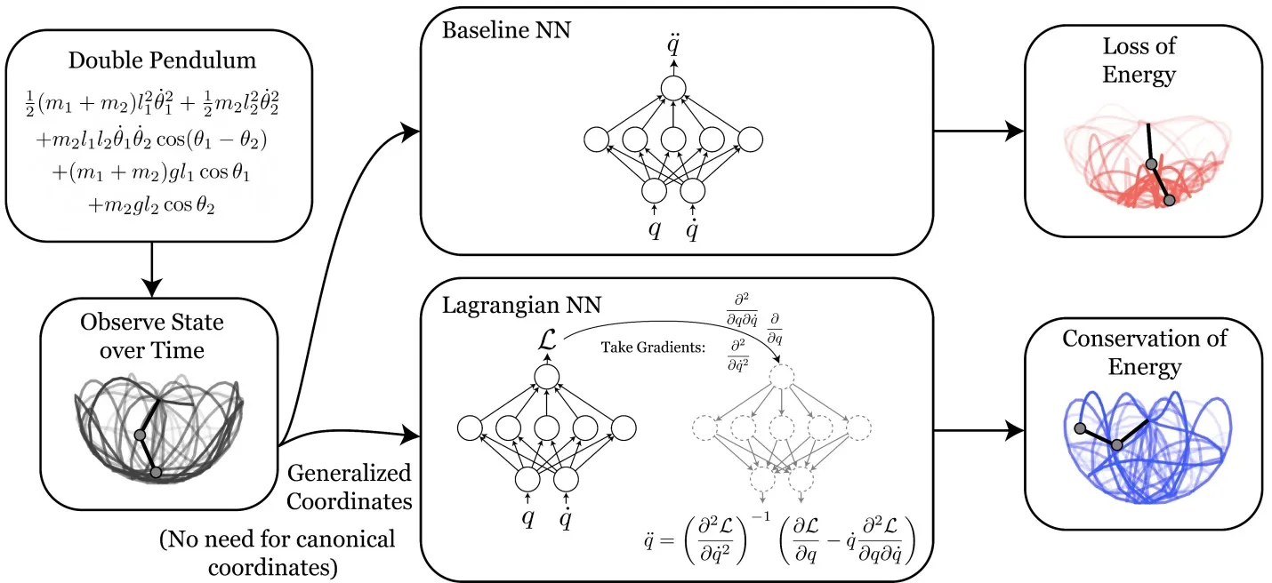Figure 2. A comparison of Lagrangian Neural Networks vs. a standard Neural Network

In figure 2, we see that, as with a Hamiltonian neural network, the Lagrangian NN performs substantially better than a standard Deep Learning NN. (Ref. https://astroautomata.com/paper/lagrangian-neural-networks/)

Integrating Hamiltonian and Lagrangian Mechanics with Neural Networks

Hamiltonian Neural Networks:

HNNs use a neural network to approximate the Hamiltonian function, ensuring that the network respects the symplectic structure of the system. The loss function is designed to minimize the discrepancy between the predicted and true dynamics, typically measured using Hamilton’s equations.

Training Process for Hamiltonian Neural Networks:

Define the Hamiltonian Function: The Hamiltonian function $H$ is parameterized as a neural network with parameters $\theta$ .
Compute Time Derivatives: Using Hamilton’s equations, compute the time derivatives $\dot{q}$ and $\dot{p}$ . $\dot{q}$ represents the change of position over time and $\dot{p}$ represents the change of momentum (i.e. the rate of change of motion) changes over time.
Minimize Loss Function: The loss function is designed to penalize errors in the predicted time derivatives:

\operatorname*{argmin}\theta \bigg \Vert \frac{d\mathbf{q}}{dt} - \frac{\partial \mathcal{H}{\theta}}{\partial \mathbf{p}} \bigg \Vert^2 ~+~ \bigg \Vert \frac{d\mathbf{p}}{dt} + \frac{\partial \mathcal{H}_{\theta}}{\partial \mathbf{q}} \bigg \Vert^2

Training Process for Lagrangian Neural Networks:

Define the Lagrangian Function: The Lagrangian function $L$ is parameterized as a neural network $L_\theta$ with parameters $\theta$ .
Compute Time Derivatives: Using the Euler-Lagrange equations, compute the time derivatives.
Minimize Loss Function: The loss function ensures that the learned Lagrangian satisfies the Euler-Lagrange equations, minimizing the discrepancy between the predicted and true dynamics.

Comparative Analysis

Similarities:

Both HNNs and LNNs integrate classical mechanics principles into neural networks.
They ensure that learned models respect fundamental physical laws, leading to more accurate and interpretable results.
Both approaches can significantly improve the modeling of dynamical systems, especially over long time periods.

Differences:

HNNs focus on learning the Hamiltonian function, ideal for systems where energy conservation is crucial.
LNNs focus on learning the Lagrangian function, advantageous for systems with constraints or where the formulation in terms of coordinates and velocities is more natural.
The mathematical formulations (Hamilton’s equations vs. Euler-Lagrange equations) lead to different training and implementation strategies.

Applications of Hamiltonian and Lagrangian Neural Networks in Finance

Hamiltonian and Lagrangian neural networks (HNNs and LNNs) offer unique advantages for modeling and predicting complex financial systems due to their ability to capture dynamic behaviors and preserve structural constraints.

Modeling Financial Systems

Dynamic Asset Pricing: HNNs and LNNs can accurately model the intricate dynamics of asset prices by learning the underlying equations governing market behavior. This ensures that key financial principles, such as the conservation of capital, are maintained. This is especially useful for modeling highly dynamic markets where traditional models may fall short.
Derivatives Pricing: These models enhance the pricing of financial derivatives by incorporating the complex, stochastic processes that drive market behaviors. By doing so, they provide more accurate and reliable pricing compared to traditional models like Black-Scholes.

Predictive Analysis

Market Trend Prediction: By leveraging conservation laws, HNNs and LNNs provide more stable and accurate predictions of market trends. This stability is crucial for making informed long-term investment decisions, as it reduces the noise and error inherent in traditional predictive models.
Volatility Forecasting: LNNs can effectively forecast market volatility by modeling the constraints and interactions within financial markets. This capability allows for better risk management and strategic planning, especially in volatile market conditions.

Optimization

Portfolio Management: HNNs optimize portfolio allocations over time by understanding the dynamic behavior of different assets. They ensure optimal asset distribution by predicting how each asset will perform under various market conditions, leading to maximized returns and minimized risks.
Algorithmic Trading: These networks can significantly enhance algorithmic trading strategies. By accurately predicting price movements and optimizing trade execution, HNNs help traders maximize their returns and exploit market inefficiencies.

Risk Management

Stress Testing: HNNs and LNNs can simulate various market conditions and their impacts on portfolios. This simulation capability is vital for stress testing and assessing how different scenarios might affect financial stability. It helps in identifying potential vulnerabilities and preparing appropriate risk mitigation strategies.
Credit Risk Modeling: These models can capture the dynamics of credit risk factors, providing a deeper understanding of credit risks. This understanding aids in making more informed decisions regarding lending, borrowing, and other credit-related activities.

Example Applications

Option Pricing Models

Traditional models like Black-Scholes can be enhanced using HNNs to incorporate more complex dynamics and constraints. This enhancement leads to more accurate pricing of options and derivatives, reflecting a more realistic market behavior.

Interest Rate Modeling

LNNs can model the evolution of interest rates, considering the constraints and interactions within the financial system. This capability provides better forecasts and strategies for managing interest rate risks, which is crucial for financial institutions and investors alike.

Asset Allocation

By understanding the dynamics of asset prices and their interactions, HNNs can optimize asset allocation in a portfolio. This optimization ensures better returns while effectively managing risks, making it a powerful tool for portfolio managers.

Hamiltonian and Lagrangian neural networks bring advanced modeling capabilities to the financial sector, allowing for more accurate predictions, better risk management, and optimized financial strategies. Their ability to preserve inherent structures and constraints makes them particularly valuable for long-term stability and accuracy in financial predictions and optimizations. As research and technology progress, the applications of these neural networks in finance are likely to expand, providing new tools for analysts, traders, and risk managers to navigate the complexities of financial markets.

Resources

Viewable Jupyter Notebook for this briefing