Fourier Neural Networks in Finance

Introduction to Fourier Neural Networks

Fourier Neural Networks (FNNs) represent a sophisticated integration of Fourier analysis and neural network architectures, emerging as a powerful tool in the fields of signal processing, time series analysis, and machine learning. These networks uniquely combine the spectral processing capabilities of Fourier transforms with the adaptive learning mechanisms of neural networks, offering a novel approach to handling complex, frequency-rich data.

At their core, FNNs leverage the Fourier transform, a fundamental technique in signal processing that decomposes a function of time or space into its constituent frequencies. The Fourier transform of a function f(t) is given by:

Where F(ω) represents the frequency domain representation of the time-domain function f(t), and ω denotes angular frequency.

In the context of neural networks, the Fourier transform is typically implemented as a layer or operation within the network architecture. This allows the network to process input data in the frequency domain, capturing periodic patterns and spectral characteristics that might be less apparent in the time domain.

The general structure of an FNN includes:

1. An input layer that accepts time-domain data
2. A Fourier transform layer that converts the input to the frequency domain
3. One or more neural network layers that process the frequency-domain data
4. An optional inverse Fourier transform layer to convert back to the time domain
5. An output layer that produces the final predictions or classifications

Mathematically, we can represent a simple FNN as:

Where:

• x is the input signal
• 𝓕 represents the Fourier transform
• 𝓕⁻¹ is the inverse Fourier transform
• Φ denotes the frequency-domain processing (which may involve multiple neural network layers)
• W and b are the weights and biases of the final layer
• σ is an activation function

In financial applications, FNNs offer several advantages:

1. Efficient processing of periodic market patterns
2. Ability to capture multi-scale temporal dependencies in financial time series
3. Enhanced feature extraction in the frequency domain, revealing hidden patterns in market data
4. Potential for improved prediction accuracy in tasks such as price forecasting and risk assessment

As we explore more deeply into the architecture and applications of FNNs, we will explore how these networks can be leveraged to address complex challenges in quantitative finance, algorithmic trading, and economic forecasting.

Theoretical Background: Fourier Transforms

Introduction to Fourier Transforms

Fourier transforms are powerful mathematical tools that allow us to decompose complex signals into simpler, periodic components. Named after the French mathematician Joseph Fourier, these transforms help us analyze and process signals in many fields, including finance.

Imagine you’re listening to a complex piece of music. Your ear naturally breaks down this sound into individual notes and instruments. A Fourier transform does something similar with mathematical signals - it breaks down a complex signal into its constituent frequencies.

The Basics of Fourier Transforms

At its core, a Fourier transform converts a signal from its original domain (often time) to the frequency domain. The mathematical representation of a continuous Fourier transform is:

Don’t worry if this looks intimidating! In simple terms, this equation takes a function f(t) (our original signal) and transforms it into F(ω), which tells us about the frequencies present in the original signal.

Discrete Fourier Transform (DFT) and Fast Fourier Transform (FFT)

In the real world, especially in finance, we often work with discrete data points rather than continuous functions. This is where the Discrete Fourier Transform (DFT) comes in:

The Fast Fourier Transform (FFT) is an efficient algorithm to compute the DFT. It dramatically reduces the computation time, making it possible to analyze large datasets quickly.

The Role of Sine and Cosine Functions in FFTs

To truly understand Fourier transforms, it’s crucial to grasp the role of sine and cosine functions. These trigonometric functions are the building blocks of Fourier analysis.

Fundamentals of Sine and Cosine

Sine and cosine are periodic functions that repeat every 2π radians (or 360 degrees). They have several key properties that make them useful for Fourier analysis:

1. They oscillate between -1 and 1.
2. They are smooth and continuous.
3. They are orthogonal to each other, meaning they are independent.

Representing Signals with Sine and Cosine

The core idea of Fourier analysis is that any periodic function can be represented as a sum of sine and cosine functions of different frequencies. Mathematically, this is expressed as:

Where:

• $f(t)$ is our signal
• $a₀$ is the average value of the function
• $aₙ$ and $bₙ$ are the amplitudes of the cosine and sine components
• ω is the fundamental frequency
• n represents the harmonics

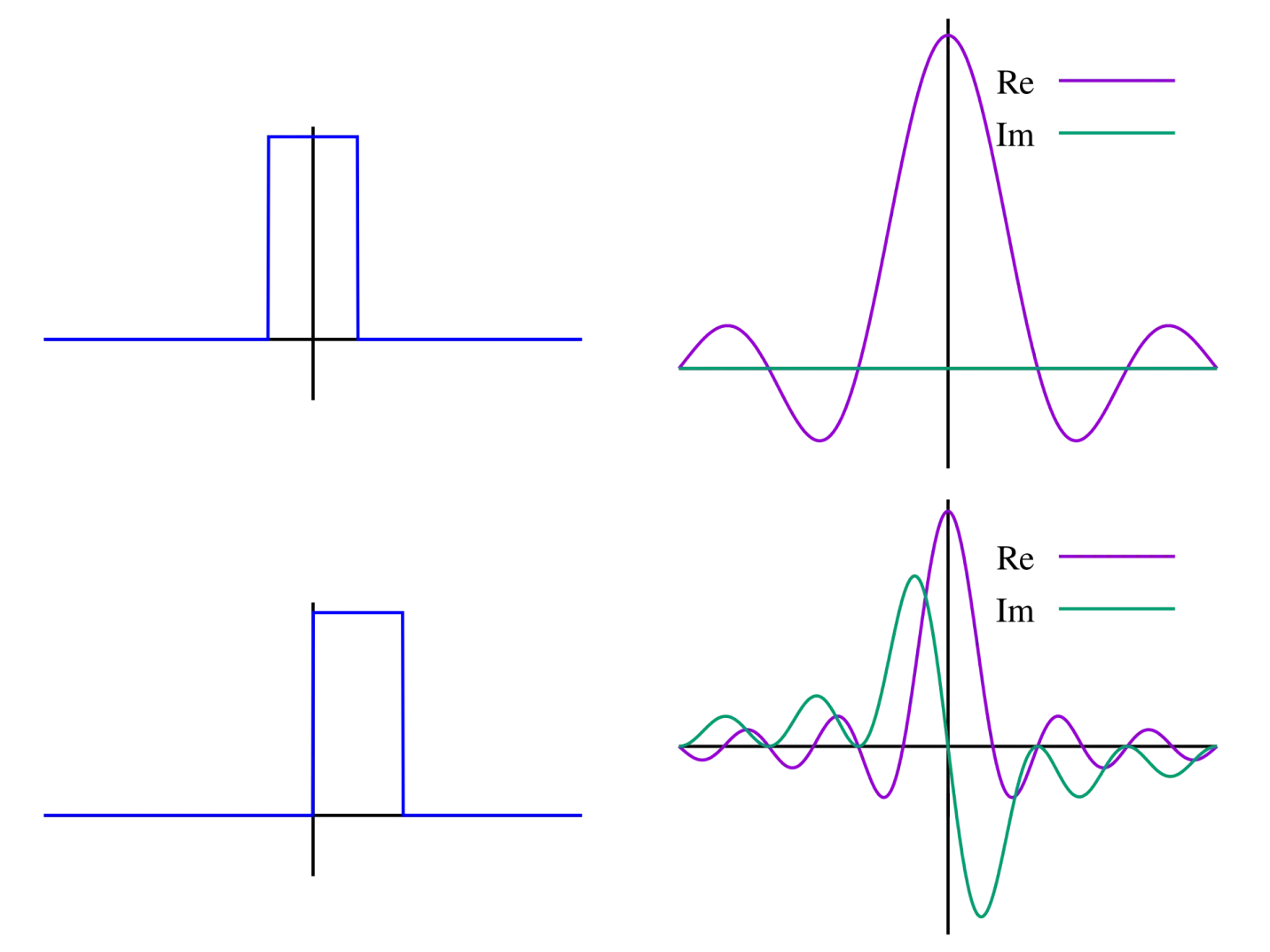Figure 1:A unit pulse as a function of time and its Fourier transformation

Complex Exponentials and Euler’s Formula

In practice, FFTs often use complex exponentials instead of explicit sines and cosines. This is based on Euler’s formula:

This allows us to represent both sine and cosine in a single complex exponential, simplifying calculations and leading to the familiar form of the Fourier transform:

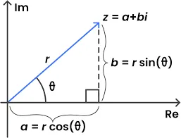Figure 2: Rewriting complex exponentials in polar coordinates rather than Cartesian coordinates

We use the exponential form to compactly represent complex exponentials.

FFTs and Frequency Components

When you apply an FFT to a signal:

1. The algorithm effectively correlates the signal with sine and cosine waves of various frequencies.
2. If the signal has a strong component at a particular frequency, the correlation with the sine and cosine at that frequency will be high.
3. The output of the FFT gives you complex numbers, where:
   • The magnitude represents the strength of that frequency component
   • The phase represents the offset of that sine/cosine component

Example in Financial Data Analysis

Let’s consider a simple example in finance:

Imagine you have daily returns of a stock over a year. You suspect there might be some weekly patterns. Here’s how sine and cosine functions in an FFT could help:

1. Apply the FFT to your daily returns data.
2. Look at the magnitude of the frequency component corresponding to a 5-day cycle (representing a week in trading days).
3. If this magnitude is significant, it suggests a weekly pattern exists.
4. The phase of this component would tell you on which day of the week the pattern tends to peak.

For instance, you might find that your stock tends to perform better towards the end of the week. This information could be valuable for timing trades or understanding market dynamics.

Visualizing Sine and Cosine in FFT Results

When you plot the results of an FFT, you’re essentially looking at how much of each frequency (represented by different sine and cosine waves) is present in your original signal. In a typical FFT plot:

• The x-axis represents frequency
• The y-axis represents the magnitude (strength) of each frequency component

A peak in this plot means your original signal has a strong component of that particular frequency, which in financial terms could represent daily, weekly, monthly, or even yearly cycles in your data.

Understanding the role of sine and cosine functions in FFTs provides deeper insight into how these transforms work and how they can reveal hidden periodicities in financial data. This knowledge can be instrumental in developing more sophisticated analysis techniques and trading strategies.

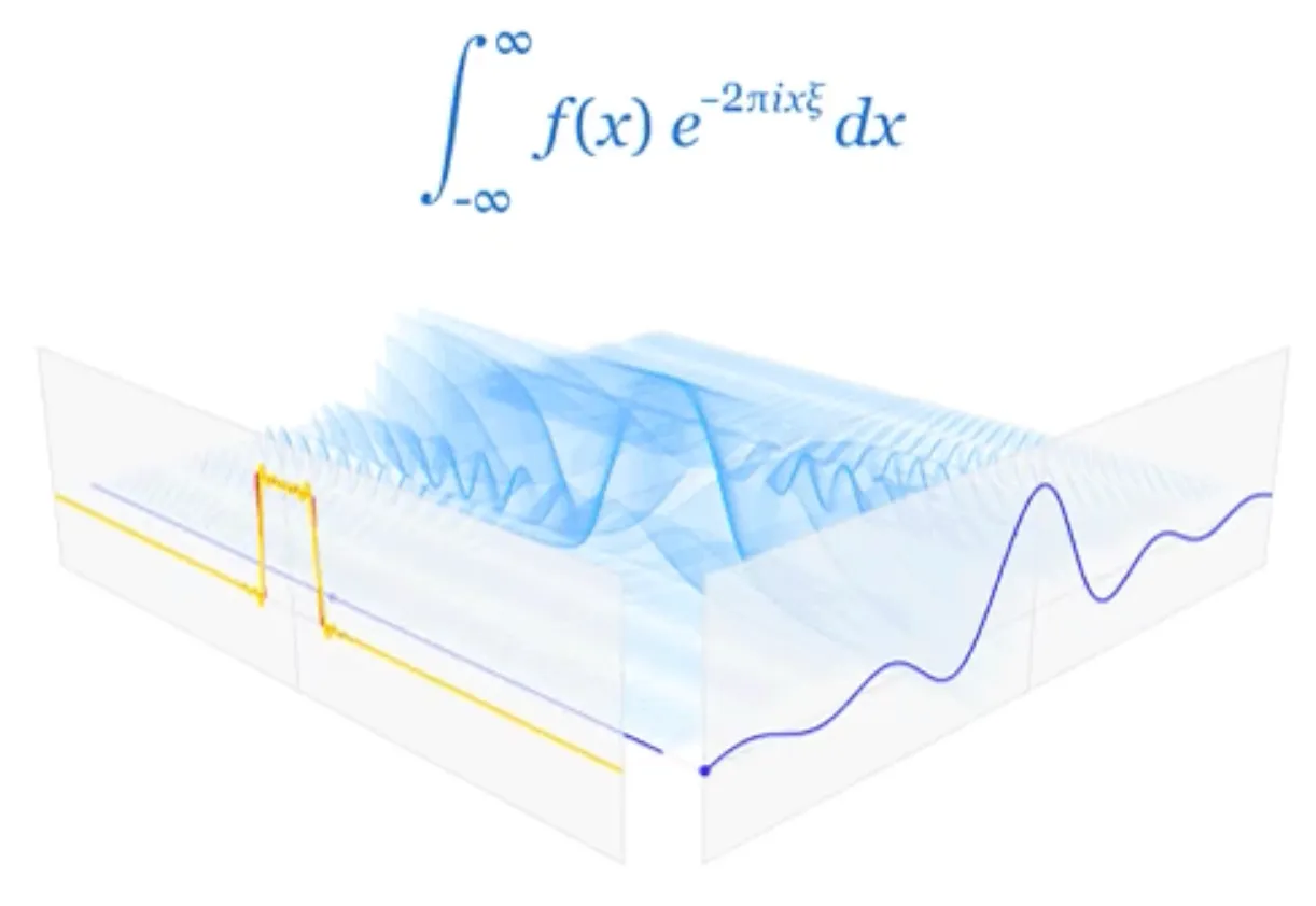Figure 3: A clear visualization of the Fourier Transform

See this Reddit post

Use Cases in Finance

Let’s explore two common use cases of Fourier transforms in finance:

Use Case 1: Market Trend Analysis

Imagine you’re an analyst trying to understand the trends in a stock’s price over the past year. You have daily closing prices, but you want to identify any recurring patterns or cycles.

Here’s how you might apply an FFT:

1. Gather the daily closing prices for the past year (let’s say 252 trading days).
2. Apply the FFT algorithm to this data.
3. The output will show you the strength of different frequencies in your data.

For example, you might find:

• A strong low-frequency component, indicating a long-term trend.
• A peak at a frequency corresponding to about 20-22 days, suggesting a monthly cycle.
• Another peak at a frequency of about 63 days, hinting at a quarterly pattern.

This analysis can help you understand the stock’s behavior and potentially forecast future movements.

Use Case 2: High-Frequency Trading Signal Processing

Now, let’s say you’re developing a high-frequency trading algorithm. You’re dealing with price data coming in every millisecond, and you want to filter out noise to identify true price movements.

Here’s how FFT can help:

1. Collect price data over a short time window (e.g., the last 1024 data points).
2. Apply the FFT to this dataset.
3. Examine the frequency components:
   • Very high-frequency components often represent noise.
   • Lower frequency components may represent actual price trends.
4. Apply a filter to remove the high-frequency noise.
5. Use the Inverse FFT to convert the filtered data back to the time domain.

This process helps clean the signal, allowing your algorithm to make decisions based on more reliable price movements rather than market noise.

Neural Networks: A Brief Review and Relevance to Fourier Neural Networks

Quick Recap of Deep Neural Networks

As a brief reminder, deep neural networks are characterized by:

1. Multiple hidden layers
2. Non-linear activation functions
3. Gradient-based learning algorithms
4. Ability to automatically learn hierarchical representations

Key Aspects Relevant to Fourier Neural Networks

When considering neural networks in the context of Fourier Neural Networks (FNNs), several aspects become particularly important:

Handling Frequency Domain Inputs

In FNNs, neural networks often operate on frequency domain representations of data. This requires careful consideration of:

1. Input layer design: The input layer must be able to handle complex-valued inputs resulting from Fourier transforms.
2. Activation functions: Traditional activation functions may need to be adapted or replaced to handle complex numbers effectively.

Spectral Pooling

Spectral Pooling vs. Spatial Pooling

Understanding the difference between spectral pooling and spatial pooling is crucial for grasping the unique advantages of Fourier Neural Networks (FNNs). Let’s dive deep into these concepts.

Spatial Pooling: A Quick Review

In traditional Convolutional Neural Networks (CNNs), spatial pooling is a common operation used to reduce the spatial dimensions of feature maps. The two most common types are:

1. Max Pooling: Selects the maximum value in each pooling window.
2. Average Pooling: Computes the average of all values in each pooling window.

Mathematically, for a 2x2 max pooling operation:

Where x is the input feature map and y is the output.

Spatial pooling has several effects:

• Reduces computational complexity
• Provides some translation invariance
• Helps in capturing hierarchical features

However, it also has limitations:

• Loss of fine-grained information
• Potential loss of important features if they don’t align with pooling windows

Figure 4: An example of spatial pooling Ref Factorized atrous spatial pyramid pooling module

Spectral Pooling: Pooling in the Frequency Domain

Spectral pooling, introduced in the context of FNNs, operates in the frequency domain rather than the spatial domain. Here’s how it works:

1. The input feature map is transformed to the frequency domain using the Discrete Fourier Transform (DFT).
2. The frequency representation is truncated, keeping only the low-frequency components.
3. The truncated frequency representation is transformed back to the spatial domain using the Inverse DFT.

Mathematically, for a 1D input signal x of length N, spectral pooling to length M (M < N) can be expressed as:

Where:

• $DFT$ is the Discrete Fourier Transform
• $IDFT$ is the Inverse Discrete Fourier Transform
• $Truncate(X, M)$ keeps the M lowest frequency components of X

Key Differences and Advantages of Spectral Pooling

1. Information Preservation:

   • Spatial pooling can lose high-frequency information indiscriminately.
   • Spectral pooling preserves low-frequency information, which often carries the most important features in many signals, including financial time series.

2. Flexibility:

   • Spatial pooling typically uses fixed window sizes (e.g., 2x2).
   • Spectral pooling can easily adjust the degree of downsampling by changing the number of frequency components retained.

3. Global Context:

   • Spatial pooling operates locally, potentially missing global patterns.
   • Spectral pooling considers the entire input, preserving global structure.

4. Aliasing:

   • Spatial pooling can introduce aliasing effects.
   • Spectral pooling naturally avoids aliasing by truncating high frequencies.

5. Reversibility:

   • Spatial pooling is not reversible; information is permanently lost.
   • Spectral pooling is partially reversible; the low-frequency components are perfectly preserved.

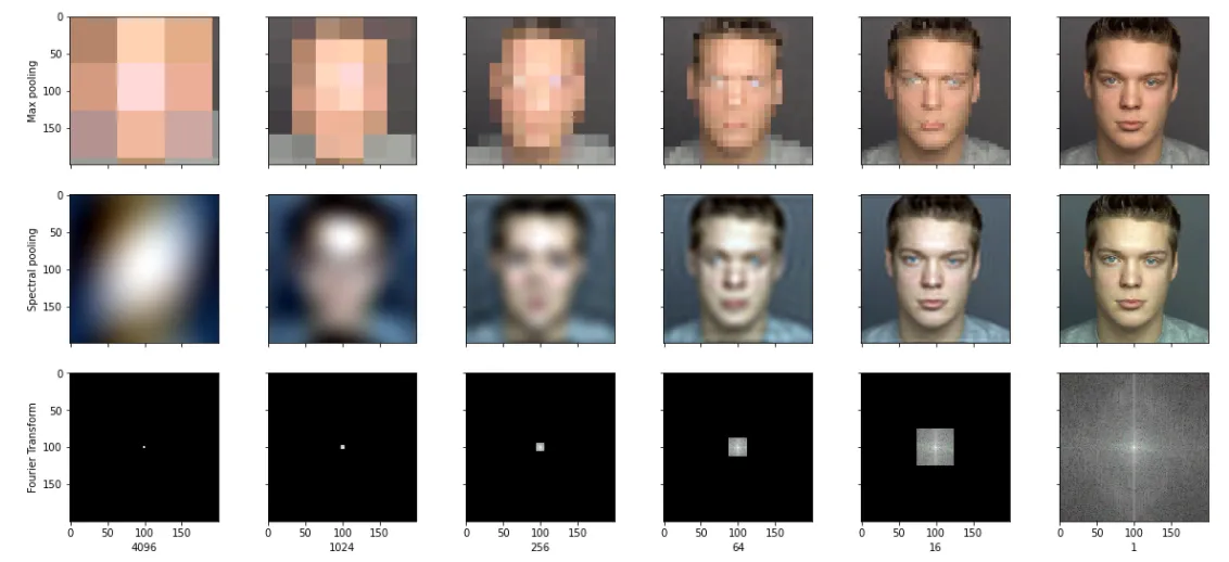Figure 5: An example of spectral pooling for RGB images in a convolutional neural network

The first row is the images after max pooling with the dimension reduction ratio described below. The second row is the image after spectral pooling with the same dimension reduction ratio applied to the spectral representation. The third row is a visualization of the frequencies that are kept after the low pass filter for the given dimension reduction ratio.

We can clearly see that the spectral pooling is much better at keeping the overall structure of the image intact through the extreme amounts of pooling.

We can see that in the most extreme case of dimension reduction (by a factor of 4096), the max pooling output has lost all resemblances to the original image but in the spectral pooling with just 8 frequencies , we can still see the silhouette of the man taking the photo.

Spectral Pooling in Financial Applications

In financial time series analysis, spectral pooling can be particularly advantageous:

1. Trend Preservation: Low-frequency components often represent long-term trends in financial data. Spectral pooling preserves these crucial features.

2. Noise Reduction: By truncating high-frequency components, spectral pooling can effectively filter out high-frequency noise, which is common in financial data.

3. Multi-scale Analysis: By varying the number of frequency components retained, spectral pooling facilitates analysis at multiple time scales, from intraday patterns to long-term trends.

4. Efficient Representation: Financial time series often have compact representations in the frequency domain. Spectral pooling capitalizes on this, allowing for efficient data compression while retaining essential information.

Complex-valued Neural Networks

Complex-valued neural networks (CVNNs) are a fundamental component of many Fourier Neural Network architectures. These networks operate on complex numbers, allowing them to process and learn from data in the frequency domain more naturally and effectively.

Complex Numbers in Neural Networks

In CVNNs, weights, biases, activations, and gradients are all complex-valued. A complex number z can be represented as:

Where a is the real part, b is the imaginary part, and i is the imaginary unit (i² = -1).

Complex-Valued Neurons

A complex-valued neuron computes its output as:

Where:

• $w_j$ are complex weights
• $z_j$ are complex inputs
• $b$ is a complex bias
• $f$ is a complex activation function

Key Components of Complex-Valued Networks

Complex Weight Initialization Algorithms for Complex-Valued Networks

Proper weight initialization is crucial for the training of neural networks, and this is especially true for complex-valued neural networks (CVNNs) used in Fourier Neural Networks (FNNs). Good initialization can lead to faster convergence, better performance, and increased stability during training.

Importance of Proper Initialization

In CVNNs, weight initialization is particularly critical because:

1. Complex-valued operations can lead to more unstable gradients.
2. The interplay between real and imaginary parts can cause issues if not properly balanced.
3. The magnitude of complex numbers can grow or shrink rapidly during forward and backward passes.

Key Considerations for Complex Weight Initialization

When initializing weights in CVNNs, we need to consider:

1. Magnitude: The overall scale of the weights.
2. Phase: The angle of the complex number in the complex plane.
3. Independence: Ensuring real and imaginary parts are initialized independently.
4. Variance: Maintaining appropriate variance of activations through the network.

Complex Weight Initialization Algorithms

Let’s explore several algorithms for initializing weights in CVNNs, along with their mathematical foundations and implementation details.

Complex Glorot/Xavier Initialization

The Glorot (also known as Xavier) initialization aims to maintain the variance of activations and gradients across layers.

Mathematical Basis: For a layer with n_in input units and n_out output units, we draw weights from a uniform distribution:

Complex He Initialization

He initialization is designed for layers with ReLU activation functions and aims to maintain the variance of activations.

Mathematical Basis: For a layer with n_in input units, we draw weights from a normal distribution:

Complex Activation Functions

Designing activation functions for complex numbers requires careful consideration. Some options include:

1. Complex ReLU:

2. Complex Tanh:

3. Complex Cardioid:

Complex Backpropagation

Backpropagation in CVNNs involves computing gradients with respect to both real and imaginary parts:

Where L is the loss function and w is a complex weight.

Advantages of Complex-Valued Networks in FNNs

1. Natural Processing of Frequency Domain Data: CVNNs can directly operate on the output of Fourier transforms without losing phase information.

2. Richer Representations: Complex numbers allow for more compact and expressive representations of certain types of data.

3. Phase Sensitivity: CVNNs can learn and utilize phase information, which is crucial in many signal processing tasks.

4. Improved Gradient Flow: The complex plane offers more pathways for gradient flow, potentially mitigating vanishing gradient problems.

Challenges and Considerations

1. Increased Computational Complexity: Complex operations are generally more computationally expensive than their real-valued counterparts.

2. Design of Activation Functions: Designing activation functions that maintain desirable properties in the complex domain is non-trivial.

3. Interpretation of Results: Complex-valued outputs may be less straightforward to interpret, especially in financial contexts.

4. Limited Software Support: While improving, many deep learning frameworks have limited native support for complex-valued operations.

Applications in Financial Data Analysis

Complex-valued networks in FNNs offer unique advantages for financial data analysis:

1. Time-Frequency Analysis: CVNNs can effectively process and learn from spectrograms or wavelet transforms of financial time series.

2. Cyclical Pattern Recognition: The ability to process phase information allows for better recognition of cyclical patterns in market data.

3. Multi-Dimensional Dependencies: Complex representations can capture intricate dependencies between different financial variables.

4. Signal Denoising: CVNNs can be effective in separating signal from noise in financial data by operating in the frequency domain.

Architectural Considerations for FNNs

When designing neural network components for FNNs, consider:

1. Hybrid architectures: Combining CNN-like structures for spectral processing with RNN/LSTM components for temporal dependencies.

2. Attention mechanisms: Implementing attention in the frequency domain to focus on relevant spectral components.

3. Residual connections: Using skip connections to facilitate gradient flow, especially important when working with phase information.

Learning in the Frequency Domain

Training neural networks on frequency domain data presents unique challenges and opportunities:

1. Interpretability: Weights learned in the frequency domain may have direct interpretations in terms of spectral properties.

2. Regularization: Spectral regularization techniques can be employed to enforce desired frequency-domain properties.

3. Data augmentation: Frequency-domain transformations can be used for data augmentation, potentially improving model generalization.

Financial Applications: Neural Network Perspective

In financial contexts, the neural network components of FNNs can be particularly useful for:

1. Multi-scale pattern recognition: Identifying patterns across different frequency bands in financial time series.

2. Non-linear frequency interactions: Capturing complex relationships between different spectral components of financial data.

3. Adaptive filtering: Learning to focus on relevant frequency components while suppressing noise.

Implementation Considerations

When implementing the neural network components of FNNs:

1. Use libraries with good support for complex number operations (e.g., TensorFlow Complex, PyTorch)

2. Consider custom layer implementations for spectral operations

3. Carefully design loss functions that account for both magnitude and phase information

Challenges and Future Directions

As Fourier Neural Networks (FNNs) continue to evolve and find applications in finance, several challenges and promising future directions emerge. Understanding these can guide researchers and practitioners in advancing the field and realizing the full potential of FNNs in financial applications.

1. Interpretability

Challenges:

• Complex-valued networks are inherently more difficult to interpret than their real-valued counterparts.
• The frequency domain representation adds another layer of abstraction, making it challenging to translate network decisions into actionable financial insights.

Future Directions:

• Develop visualization techniques for complex-valued network activations and weights in the context of financial data.
• Create methods to map frequency-domain features back to time-domain financial indicators.
• Investigate the use of attention mechanisms in the frequency domain to highlight which spectral components are most influential in decision-making.

2. Scalability

Challenges:

• FFT operations can be computationally intensive, especially for high-frequency financial data.
• Training complex-valued networks on large financial datasets can be time-consuming and resource-intensive.

Future Directions:

• Explore optimized implementations of FFT for specific financial data structures.
• Investigate pruning and quantization techniques for complex-valued networks to reduce computational overhead.
• Develop distributed training algorithms specifically designed for FNNs in financial applications.

3. Adaptive Architectures

Challenges:

• Financial markets are non-stationary, with patterns and relationships changing over time.
• Fixed FNN architectures may not adapt well to sudden market shifts or regime changes.

Future Directions:

• Develop dynamic FNN architectures that can adjust their structure based on changing market conditions.
• Explore the use of meta-learning techniques to enable rapid adaptation to new market regimes.
• Investigate hybrid models that combine FNNs with adaptive filtering techniques from signal processing.

4. Integration with Other Techniques

Challenges:

• FNNs, while powerful, may not capture all aspects of financial systems on their own.
• Integrating FNNs with other advanced techniques without losing their spectral processing advantages can be complex.

Future Directions:

• Combine FNNs with reinforcement learning for adaptive trading strategies that leverage frequency-domain insights.
• Integrate causal inference techniques with FNNs to better understand cause-effect relationships in financial time series.
• Explore the synergy between FNNs and graph neural networks for analyzing interconnected financial systems.

5. Regulatory Compliance and Explainability

Challenges:

• Financial regulators increasingly demand explainable AI models.
• The complexity of FNNs, especially in the frequency domain, can make them appear as “black boxes” to regulators and stakeholders.

Future Directions:

• Develop explainable AI techniques specifically for FNNs in finance, possibly leveraging the interpretability of frequency components.
• Create standardized reporting methods for FNN-based financial models that satisfy regulatory requirements.
• Investigate ways to provide confidence intervals or uncertainty estimates for FNN predictions in financial contexts.

6. Handling Multi-Modal Financial Data

Challenges:

• Financial decision-making often involves diverse data types beyond just time series (e.g., text, images, network data).
• Integrating these diverse data types with the frequency-domain processing of FNNs is non-trivial.

Future Directions:

• Develop architectures that can process multi-modal financial data, combining FNNs for time series with other specialized networks for different data types.
• Explore ways to represent non-time series data in forms amenable to spectral processing.
• Investigate cross-modal attention mechanisms that can relate frequency-domain features to features from other data modalities.

7. Long-Term Dependencies and Memory

Challenges:

• Financial time series often exhibit very long-term dependencies that can be challenging to capture.
• Balancing the processing of both short-term and long-term patterns in the frequency domain is complex.

Future Directions:

• Develop specialized FNN architectures that can efficiently handle multi-scale temporal dependencies in financial data.
• Explore the use of persistent memory mechanisms in FNNs to capture long-term market trends.
• Investigate hierarchical FNN structures that process different frequency bands at different time scales.

8. Robustness and Stability

Challenges:

• Financial markets can be volatile, with extreme events that may destabilize model performance.
• Ensuring consistent performance of FNNs across various market conditions is crucial for practical applications.

Future Directions:

• Develop robust training techniques for FNNs that can handle outliers and extreme events in financial data.
• Investigate the use of adversarial training to improve the stability of FNNs in volatile market conditions.
• Explore ensemble methods that combine multiple FNNs to enhance stability and performance.

Conclusion

The field of Fourier Neural Networks in finance is ripe with challenges and opportunities. Addressing these challenges will require interdisciplinary efforts, combining insights from deep learning, signal processing, finance, and regulatory compliance.

As these challenges are tackled, FNNs have the potential to revolutionize financial modeling and decision-making, offering new levels of insight into the complex, cyclical nature of financial systems. The future directions outlined here provide a roadmap for researchers and practitioners to advance the field, promising more accurate, interpretable, and robust financial models in the years to come.